Below I present the theory and derivation as to how I arrived at the expected value of 11 collisions (+/- 3) as mentioned in my posts discussing string distance analysis (here and here). I’ve tried to make the derivation below as digestible as possible, with accessible references, but it is admittedly still a very technical read. I think its important to “show my work” on the subject, though, and I present it here and am happy to take comments and criticism (contact).
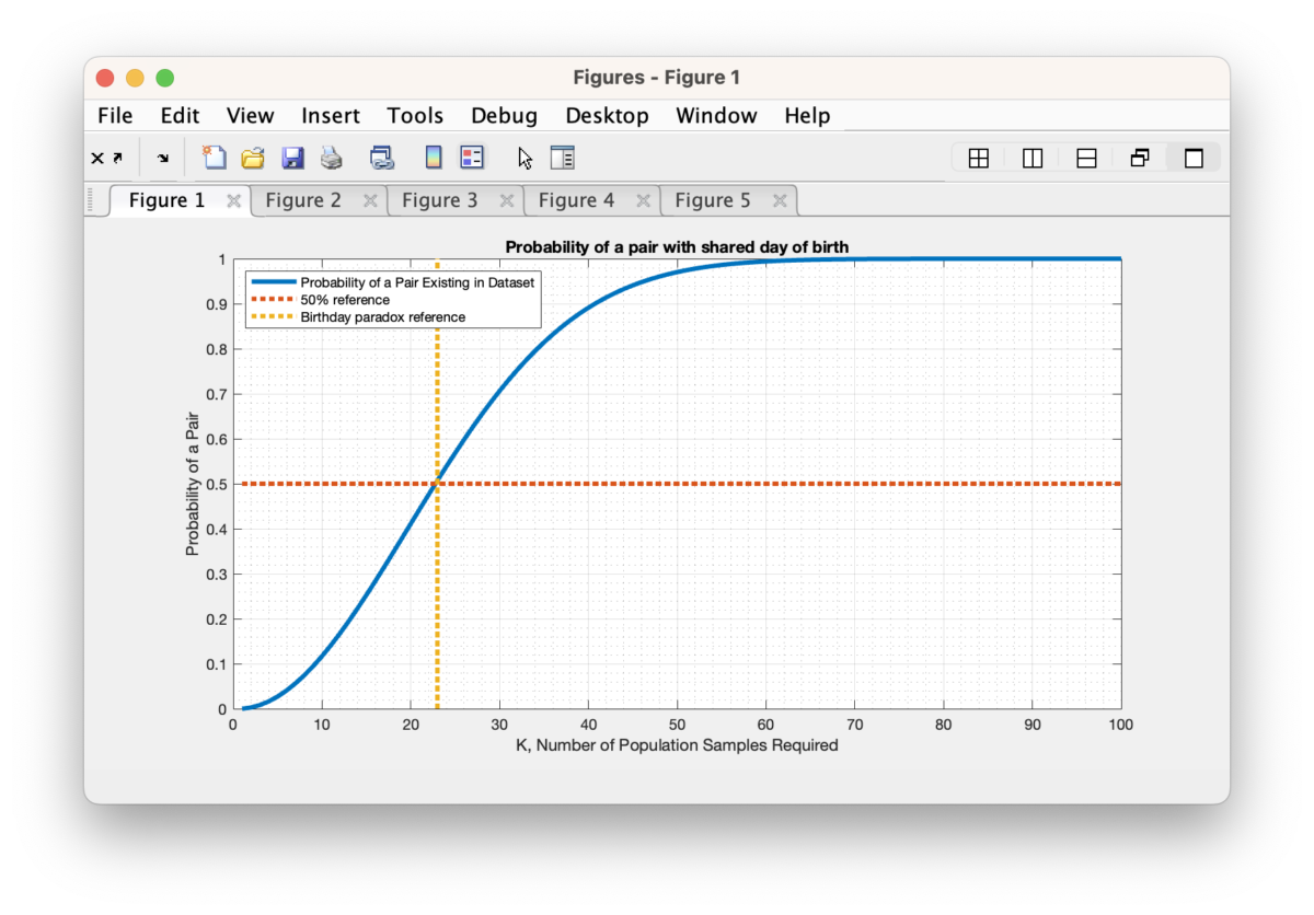
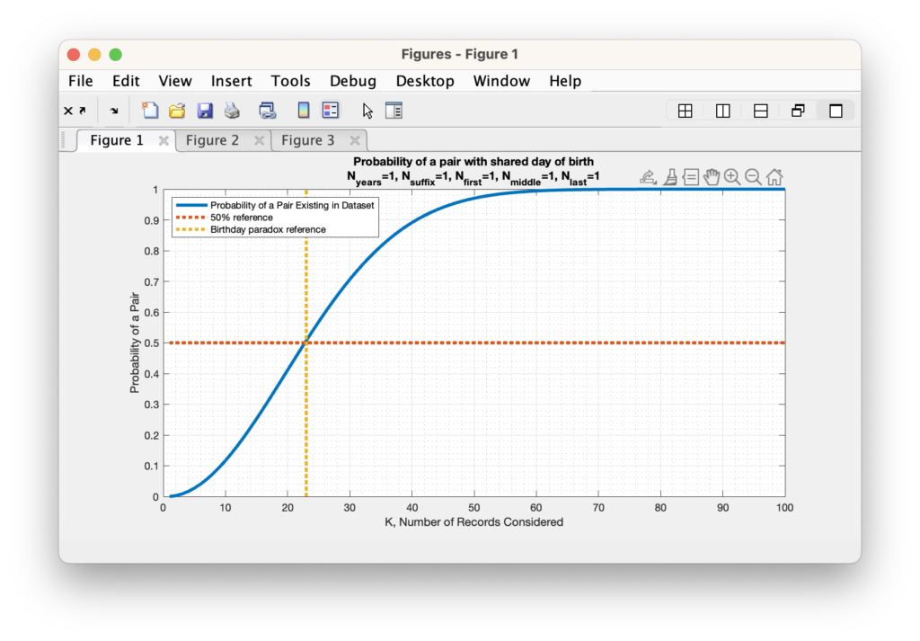
Q: How much of a chance do we actually have of getting an exact (Hamming distance of 0) collision in the full name and full date of birth? Well, there is a similar and well known probability puzzle that asks how many random people do you need to approximately have a 50% chance of 2 of them sharing the same birthday (not including the year of birth). This is known as the “Birthday Problem” in probability theory, and rather surprisingly, the answer is that you only need about 23 people in your population sample to have a 50% probability that 2 of those people will share a day-of-year of birth. To quote the wikipedia article on the matter “… While it may seem surprising that only 23 individuals are required to reach a 50% probability of a shared birthday, this result is made more intuitive by considering that the birthday comparisons will be made between every possible pair of individuals. With 23 individuals, there are 23 × 22/2 = 253 pairs to consider, far more than half the number of days in a year.” The same mathematics of the birthday problem is the basis of the Birthday Attack cryptographic exploit, and it is therefore a well-studied problem in cryptography and cyber security.
Now, as interesting as the toy birthday problem is as described above, it is over simplified for the problem we are looking at here. Firstly, the problem setup assumes independent and identically distributed random variable (e.g. an “IID” set of variables). While this is not exactly the case, the IID assumption provides for a computable first order estimate, and in the case of the classical birthday problem the estimate has been shown to be fairly accurate under experimental conditions.
Secondly, when we start additionally considering the year of birth, or sharing of first names, middle names and last names, things get much more complicated to compute, but the method is the same. We want to determine the probability of 2 people sharing the same First Name, Middle Name, Last Name, Suffix, Month-of-Birth, Day-of-Birth and Year-of-Birth in the population of unique registrants in the Registered Voter List. This means that in addition to the 365 day-of-birth possibilities, we need to estimate the number of possible years to cover, the number of possible first names, the number of possible middle names, the number of possible last names, the number of possible suffix strings and then include these possibilities into the same formulation as the birthday problem setup.
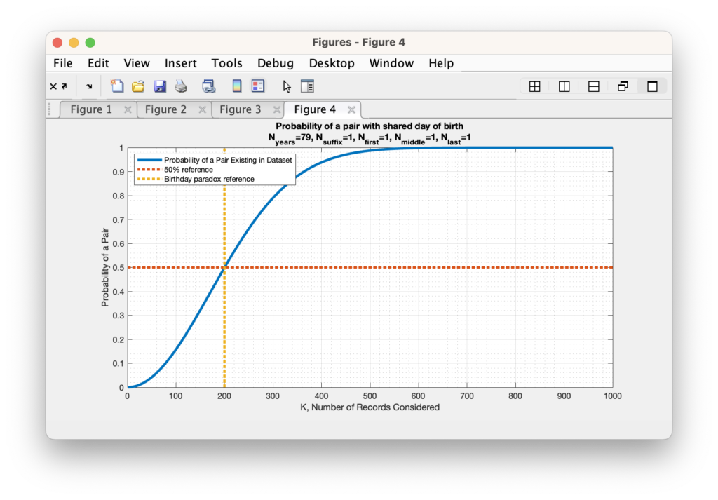
For determining how many years we should cover, I will simply use the average life expectancy of approximately 79 years. We can therefore update our N value of the birthday problem from 365 to 365 * 79 = 28835. When we perform the same analysis as the standard birthday problem with just this new parameter included, we end up needing 200 people in our sample population to have a 50% probability of of 2 people having a match.
A similar analysis can be done with the number of names being considered, etc. For each (assumed independent and uniform) variable we add to the setup, we multiply the number of possible states (N) by the number of unique variable settings.
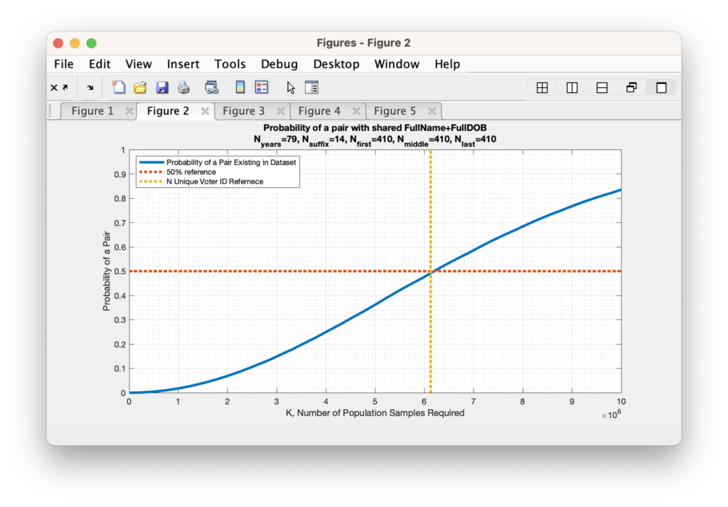
We can estimate the universe of possible names using the frequentist method from the RVL data itself: We know that we have 6,127,859 unique voter ID’s in the RVL, and there are 14 unique SUFFIX entries, 291,368 unique FIRST names, 405,591 unique MIDDLE names, and 465,185 unique LAST names. So multiplying out 365 x 79 x 14 x 291368 x 405591 x 465185 = 2.22 x 10^22 potential states to consider.
Now unfortunately, as we start dealing with bigger and bigger N values the ability of computers to maintain the necessary precision to carry out the mathematics for direct computation becomes harder and harder, eventually resulting in Infinite or divide-by-zero answers as the probabilities get smaller and smaller. So lets begin by first determining if we can find the 50% crossover point for the unique voter ID population size. We find that we only need 410 unique First, Middle, and Last names (each) to break the 50% probability limit.
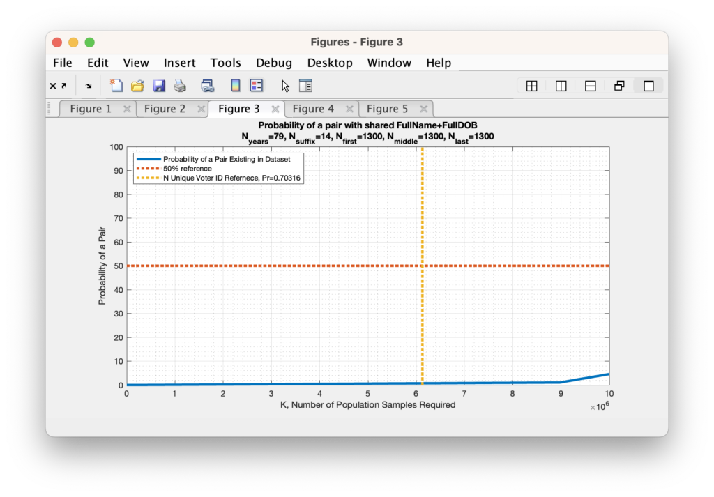
As we increase the number of unique (first, middle, last) names under consideration, we find that we very quickly reduce the probability to near zero (again … this is assuming an IID set of variables … more on that later). In fact we only need to assume that there are 1300 unique first names, middle names and last names before the probability drops to under 1%. This is two full orders of magnitude below the actual number of unique first names, middle names and last names (each) that we find by simple examination of the RVL file, so the actual probability of a collision under these conditions should be much, much, much lower. While not exactly zero, it is computationally indistinguishable from zero given machine precision. Note (again) that this formulation is still simplified in that it assumes a uniform distribution within the N possible states, but it still serves to give a first order approximation and sanity check.
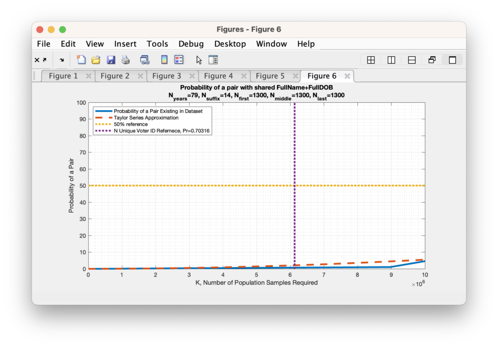
As we start approaching the limit of computational precision we have to resort to approximation methods for computing the very small, but non-zero probability of collision given the actual number of unique first, middle and last names observed in the RVL dataset. We can use the Taylor series expansion for small powers in order to do this, and our equation for computing the probability becomes: Pb = 1 – exp(-k*(k-1) / (2 *N)).
Replicating our earlier example in Figure 4 above with Nfirst == Nmiddle == Nlast == 1300 to show the comparison of the Taylor expansion to the explicit computation produces the graphic in Figure 5 below. We see that the small value approximation is close, but slightly over-estimates the directly computed probability for IID variables.
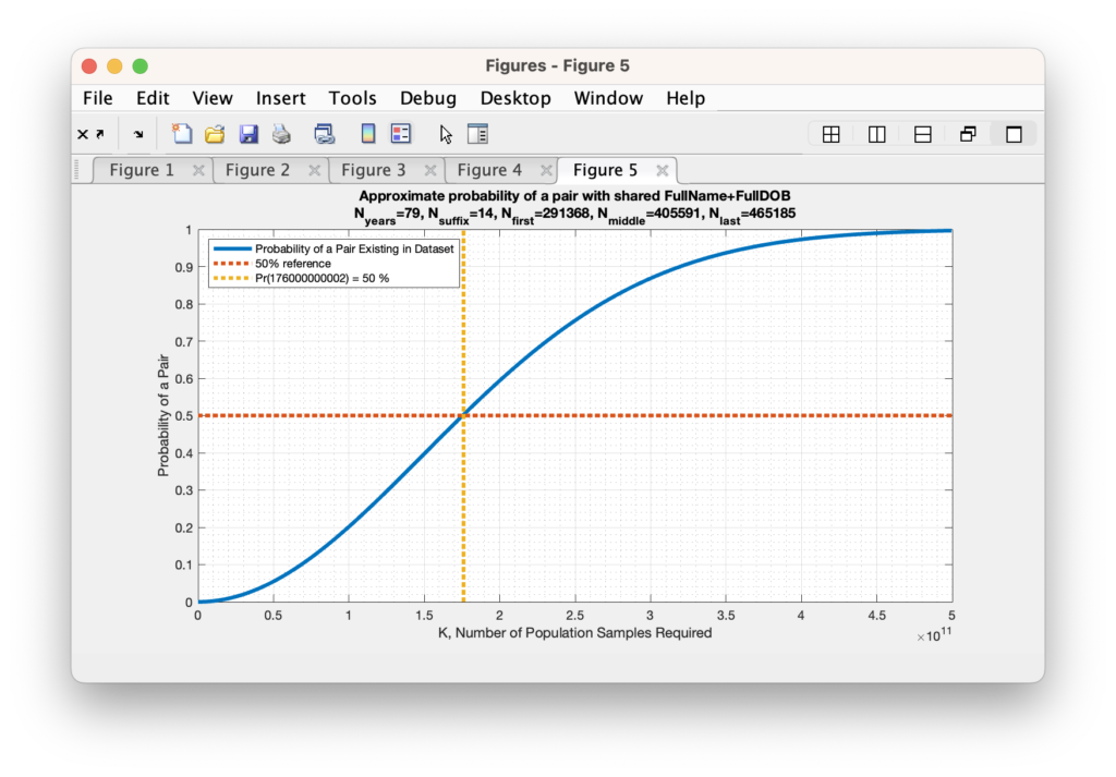
When we perform this Taylor series approximation and look to find the number of records required in order to obtain a 50% probability that any 2 records would match given our updated universe of possible matches, we end up with requiring K = 176,000,000,000, or 176 Billion records. When we again try to evaluate the Taylor series for the explicit number of unique Voter ID’s present in the RVL file, which is just over 6M, we again obtain a number that is computationally indistinguishable from 0. (To be absolutely meticulous … its a bigger number that is indistinguishable from 0 than we previously computed, but it is still indistinguishable from zero.)
Another Implementation note: In order to explicitly code the above direct computations we also need to do some clever tricks with logarithms in order to avoid numerical overflow / underflow issues as much as possible. The formula for computing the permutations, which is N! / (N-K)! = N x (N-1) x … x (N-K+1) can have numerical issues when N becomes large. However if we take the base-10 logarithm of the equation, we can use the product and quotient rules of logarithms to compute the result and avoid numerical overflow: log10( N! / (N-K)! ) = log10(N!) – log((N-K)!) = log10(N) + log10(N-1) + … + … log10(N-K+1), which is a much more stable computation.
We can perform a similar trick in order to compute the denominator of N^k by using the power property of logarithms such that log10( N^k ) = k x log10(N).
You must of course remember to reverse the logarithm once you’ve computed the log-sums. So the final computation of Pb becomes the following:
Vnr = log10(N) + log10(N-1) + … + … log10(N-K+1), where N is the number of possible states N = 365 x Nyears x Nfirst x Nmiddle x Nlast x Nsuffix.
Vt = k x log10(N)
Pa_log10 = Vnr – Vt = log10(Pa) = log10(Vnr/Vt)
Pb = 1 – 10^(Pa)
Updating from uniform distributions to non-uniform distributions
So what happens when we take into account the fact that names and birthdays are not uniformly distributed? (e.g. the last name of “Smith” is more frequent than “Sandeval”) This fact increases the probability of a collision occurring in the dataset. This increase also makes intuitive sense as we can anecdotally observe that coincident names and birthdates, while still rare … do actually happen in real life with common names.
However, in the non-uniform case we don’t have as nearly of a nice closed set of formulas for computing the probability. What we can do instead to estimate the probability is perform a number of Monte Carlo simulations of selecting K values from the weighted possibilities, and determine how many collisions occurred in each simulation trial. By setting K equal to the number of unique Voter ID values in the RVL dataset, we can directly answer the question via simulation of “how many collisions of First+Middle+Last+Suffix+DOB should we expect when looking at the VA Registered Voter List file“?
We can determine the weightings for each variable easily enough from the distributions of unique values in the data itself.
The below MATLAB weightedCollisionSim(…) function is a program that can be used to perform this analysis. It assumes that the RVL table object is a global variable to setup the trials, and uses the MATLAB built-in randsample(…) function to perform each draw.
After 100 simulation runs, the results are that for the K=6,127,859 unique voter ID’s in the RVL, we should expect to have an average of about 11 collisions at Hamming distance of 0, with a standard deviation of roughly 3.
I will note that as a validation and verification step, the MATLAB simulation code below, when used with uniform sampling, produces similar results to what we analytically derived above.
function [p,m,s] = weightedCollisionSim(k,ntrials,varargin)
% To compute the probability the ntrials must be >> 1:
% [p,m,s] = weightedCollisionSim(k,ntrials,values1,weights1,...,values2,weights2)
% [p,m,s] = weightedCollisionSim(k,ntrials,Nvalues1,weights1,...,Nvalues2,weights2)
%
% OUTPUTS:
% p = Probability of a collision
% m = mean number of collisions
% s = standard deviation of collisions

if nargin == 0
    global rvl; % Assume the RVL is an available global var

    ntrials = 100; % Number of trials

    % Population size set as num of unique voter IDs in RVL
    npop = numel(unique(rvl.IDENTIFICATION_NUMBER));

    % Convert the DOB strings to datetime objects
    dob = datetime(rvl.DOB);

    % How many unique days of the year are there?
    [ud,uda,udb] = unique(day(dob,'dayofyear'));
    % How often do they occur?
    nud = accumarray(udb,1,[numel(ud),1]);
    Ndays = numel(ud);

    % How many unique years of birth are there?
    [uy,uya,uyb] = unique(year(dob));
    % How often do they occur?
    nuy = accumarray(uyb,1,[numel(uy),1]);
    Nyears = numel(uy);

    % How many unique suffix strings are there?
    [us,usa,usb] = unique(rvl.SUFFIX);
    % How often do they occur?
    nus = accumarray(usb,1,[numel(us),1]);
    Nsuffix = numel(us);

    % How many unique first names are there?
    [uf,ufa,ufb] = unique(rvl.FIRST_NAME);
    % How often do they occur?
    nuf = accumarray(ufb,1,[numel(uf),1]);
    Nfirst = numel(uf);

    % How many unique middle names are there?
    [um,uma,umb] = unique(rvl.MIDDLE_NAME);
    % How often do they occur?
    num = accumarray(umb,1,[numel(um),1])
    Nmiddle = numel(um);

    % How many unique last names are there?
    [ul,ula,ulb] = unique(rvl.LAST_NAME);
    % How often do they occur?
    nul = accumarray(ulb,1,[numel(ul),1]);
    Nlast = numel(ul);

    % Initializing the weighting vectors
    w0 = nus;
    w1 = nud;
    w2 = nuy;
    w3 = nuf;
    w4 = num;
    w5 = nul;

    % Recursively compute results and return
    [p,m,s] = weightedCollisionSim(npop,ntrials,1:Nsuffix,w0,1:Ndays,w1,1:Nyears,w2,...
        1:Nfirst,w3,1:Nmiddle,w4,1:Nlast,w5);
    return
end

if nargin < 2 || isempty(ntrials)
    ntrials = 1;
end

nc = zeros(ntrials,1);
for j = 1:ntrials
    fprintf('Trial %d\n',j);
    y = zeros(k,numel(varargin)/2);
    m = 1;
    for i = 1:2:numel(varargin)
        w = varargin{i+1};
        v = varargin{i};
        if ~isempty(w) && isvector(w)
            % Non-uniform weightings
            y(:,m) = randsample(v,k,true,w);
        else
            % Uniform sampling
            y(:,m) = randsample(v,k,true);
        end
        m = m+1;
    end
    [u,~,ib] = unique(y,'rows');
    nu = accumarray(ib,1,[size(u,1),1]);
    nc(j) = sum(nu > 1);
end
p = mean(nc>0);
m = mean(nc);
s = std(nc);