Since I posted my initial analysis of the Henrico CVR data, one comment was made to me by a member of the Texas election integrity group I have been working with: We have been assuming, based on vendor documentation and the laws and requirements in various states, that when a cast vote record is produced by vendor software the results are sorted by the time the ballot was recorded onto a scanner. However, when looking at the results that we’ve been getting so far and trying to figure out plausible explanations for what we were seeing, he realized it might be the case that the ordering of the CVR entries are being done by both time AND USB stick grouping (which is usually associated with a specific scanner or precinct) but then simply concatenating all of those results together.
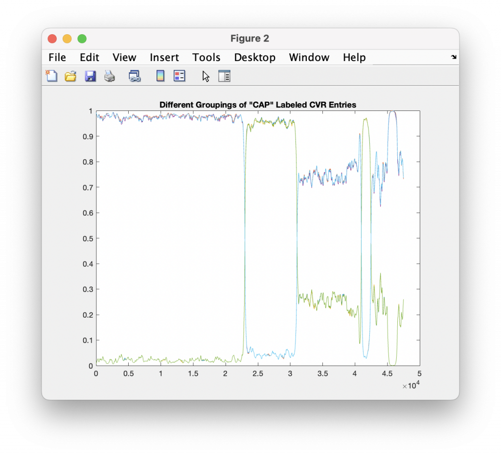
While there isn’t enough information in the Henrico CVR files to breakout the entries by USB/Scanner, and the Henrico data has record ID numbers instead of actual timestamps, there is enough information to break out them by Precinct, District and Race, with the exception of the Central Absentee Precincts (CAP) entries where we can only break them out by district given the metadata alone. However, with some careful MATLAB magic I was able to cluster the results marked as just “CAP” into at least 5 different sub-groupings that are statistically distinct. (I used an exponential moving average to discover the boundaries between groupings, and looking at the crossover points in vote share.) I then relabeled the entries with the corresponding “CAP 1”, “CAP 2”, … , “CAP 5” labels as appropriate. My previous analysis was only broken out by Race ID and CAP/Non-CAP/Provisional category.
Processing in this manner makes the individual distributions look much cleaner, so I think this does confirm that there is not a true sequential ordering in the CVR files coming out of the vendor software packages. (If they would just give us the dang timestamps … this would be a lot easier!)
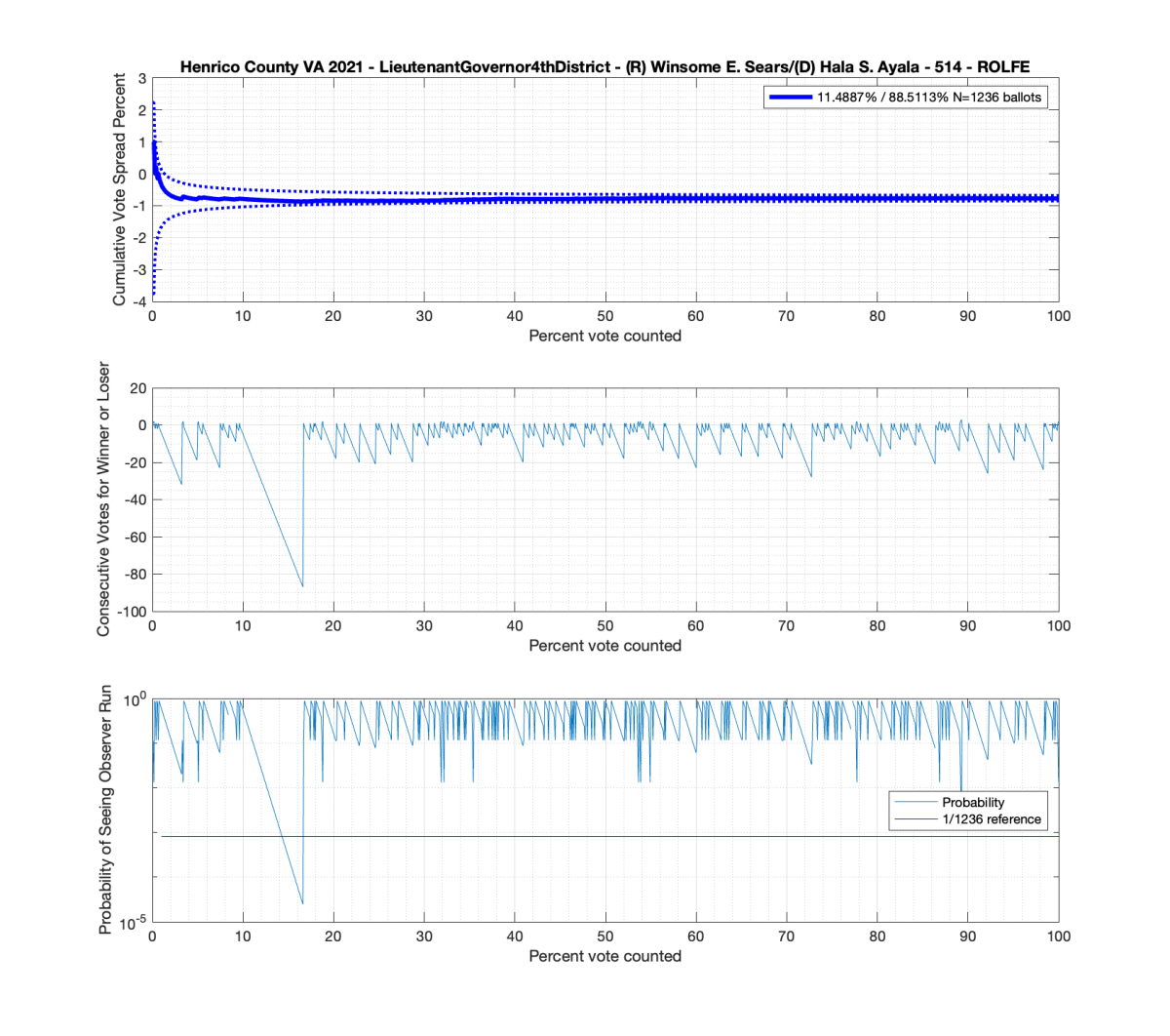
I have also added a bit more rigor to the statistics outlier detection by adding plots of the length of observed runs (e.g. how many “heads” did we get in a row?) as we move through the entries, as well as the plot of the probability of this number of consecutive tosses occurring. We compute this probability for K consecutive draws using the rules of statistical independence, which is P([a,a,a,a]) = P(a) x P(a) x P(a) x P(a) = P(a)^4. Therefore the probability of getting 4 “heads” in a row with a hypothetical 53/47 weighted coin would be .53^4 = 0.0789. There are also plotted lines for a probability 1/#Ballots for reference.
Results
The good news is that this method of slicing the data and assuming that the Vendor is simply concatenating USB drives seems to produce much tighter results that look to obey the expected IID distributions. Breaking up the data this way resulted in no plot breaking the +/- 3/sqrt(N-1) boundaries, but there still are a few interesting datapoints that we can observe.
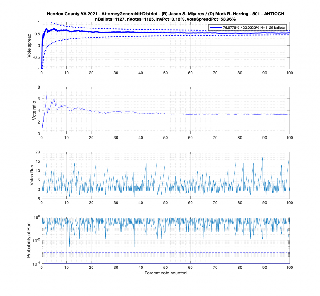
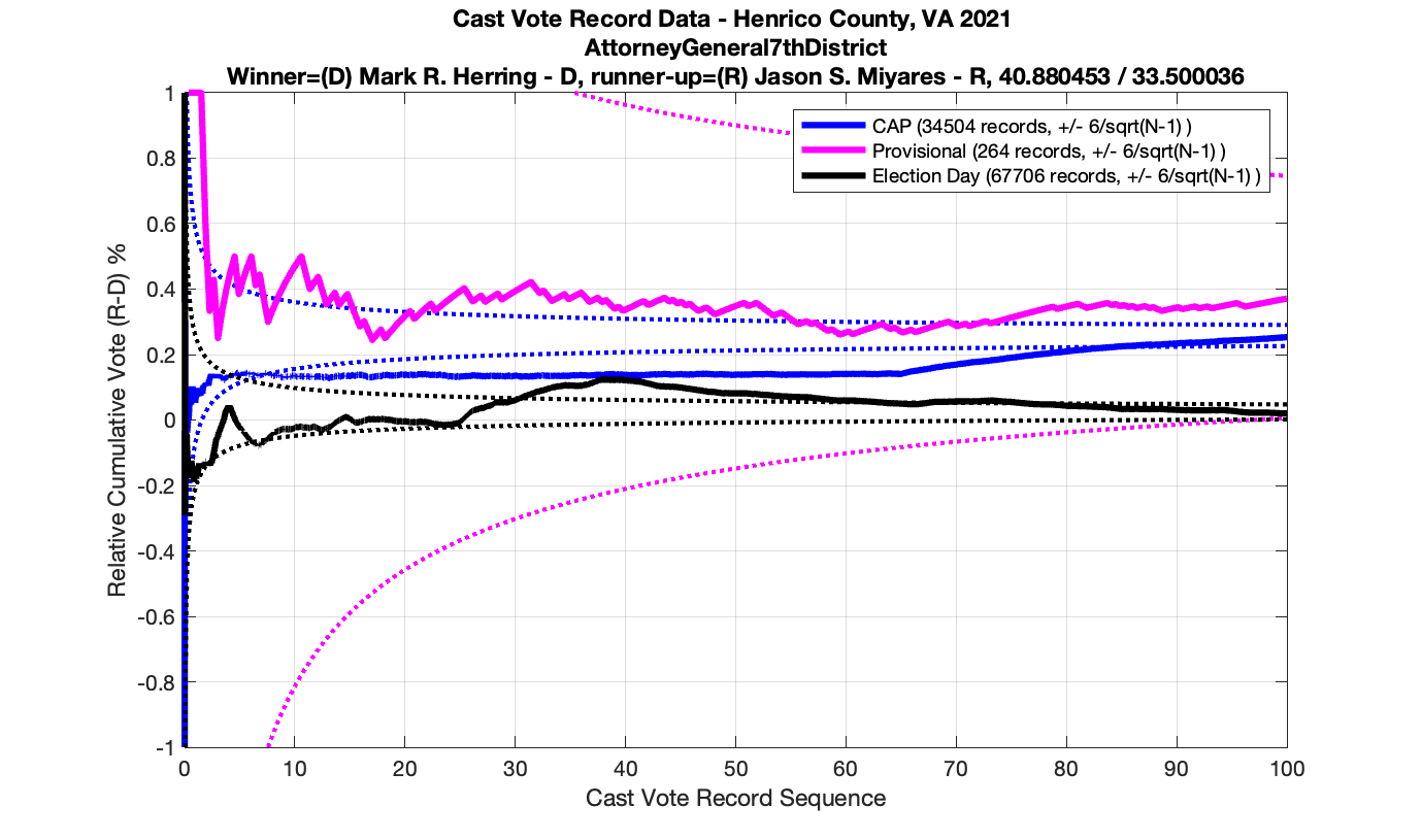
In the plot below we have the Attorney Generals race in the 4th district from precinct 501 – Antioch. This is a district that Miyares won handily 77%/23%. We see that the top plot of the cumulative spread is nicely bounded by the +/- 3/sqrt(N-1) lines. The second plot from the top gives the vote ratio in order to compare with the work that Draza Smith, Jeff O’Donnell and others are doing with CVR’s over at Ordros.com. The second from bottom plot gives the number k of consecutive ballots (in either candidates favor) that have been seen at each moment in the counting process. And the bottom plot raises either the 77% or 23% overall probability to the k-th power to determine the probability associated with pulling that many consecutive Miyares or Herring ballots from an IID distribution. The most consecutive ballots Miyares received in a row was just over 15, which had a .77^15 = 0.0198 or 1.98% chance of occurring. The most consecutive ballots Herring received was about 4, which equates to a probability of occurrence of .23^4 = 0.0028 or 0.28% chance. The dotted line on the bottom plot is referenced at 1/N, and the solid line is referenced at 0.01%.
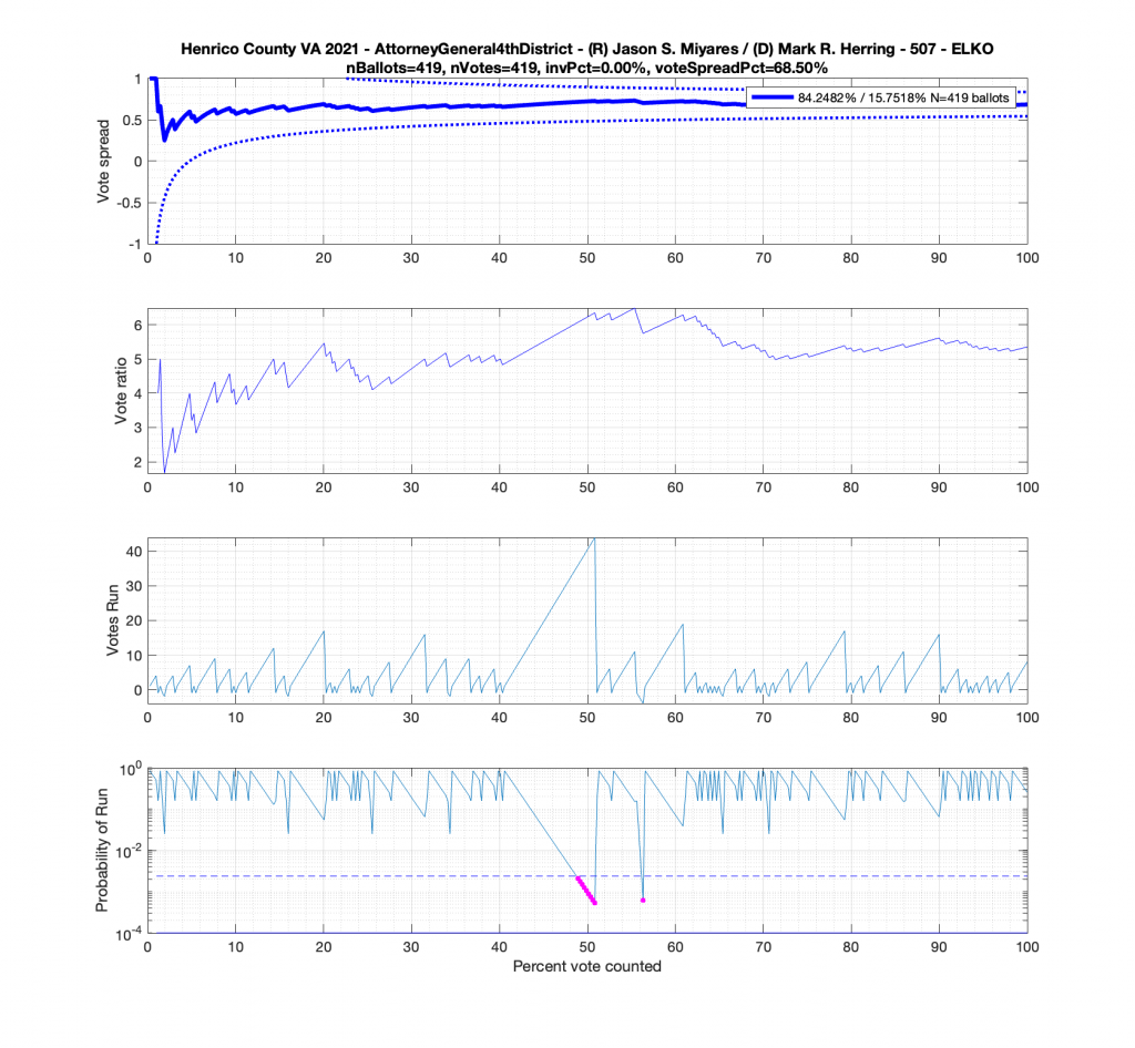
But let’s now take a look at another plot for the Miyares contest in another blowout locality with 84% / 16% for Miyares. The +/- 3/sqrt(N-1) limit nicely bounds our ballot distribution again. There is, however, an interesting block of 44 consecutive ballots for Miyares about halfway through the processing of ballots. This equates to .84^44 = 0.0004659 or a 0.04659% chance of occurrence from an IID distribution. Close to this peak is a run of 4 ballots for Herring which doesn’t sound like much, but given the 84% / 16% split, the probability of occurrence for that small run is .16^4 = 0.0006554 or 0.06554%!
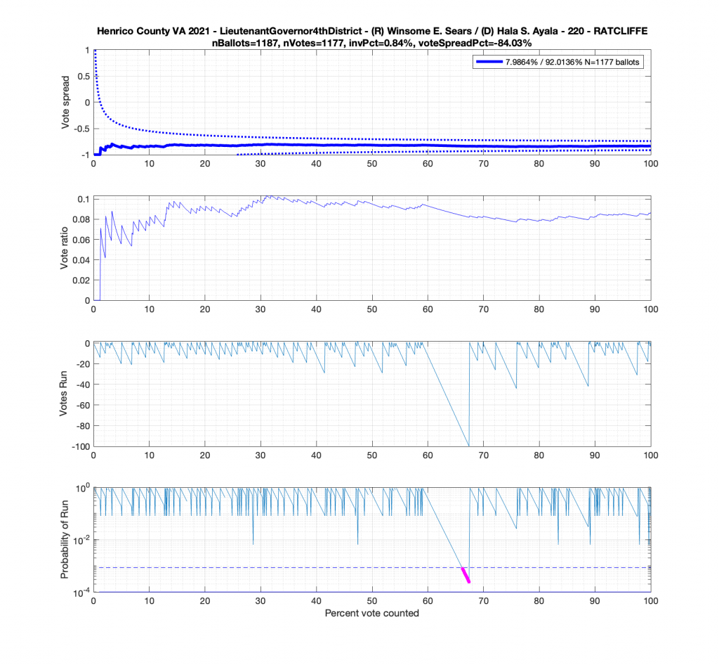
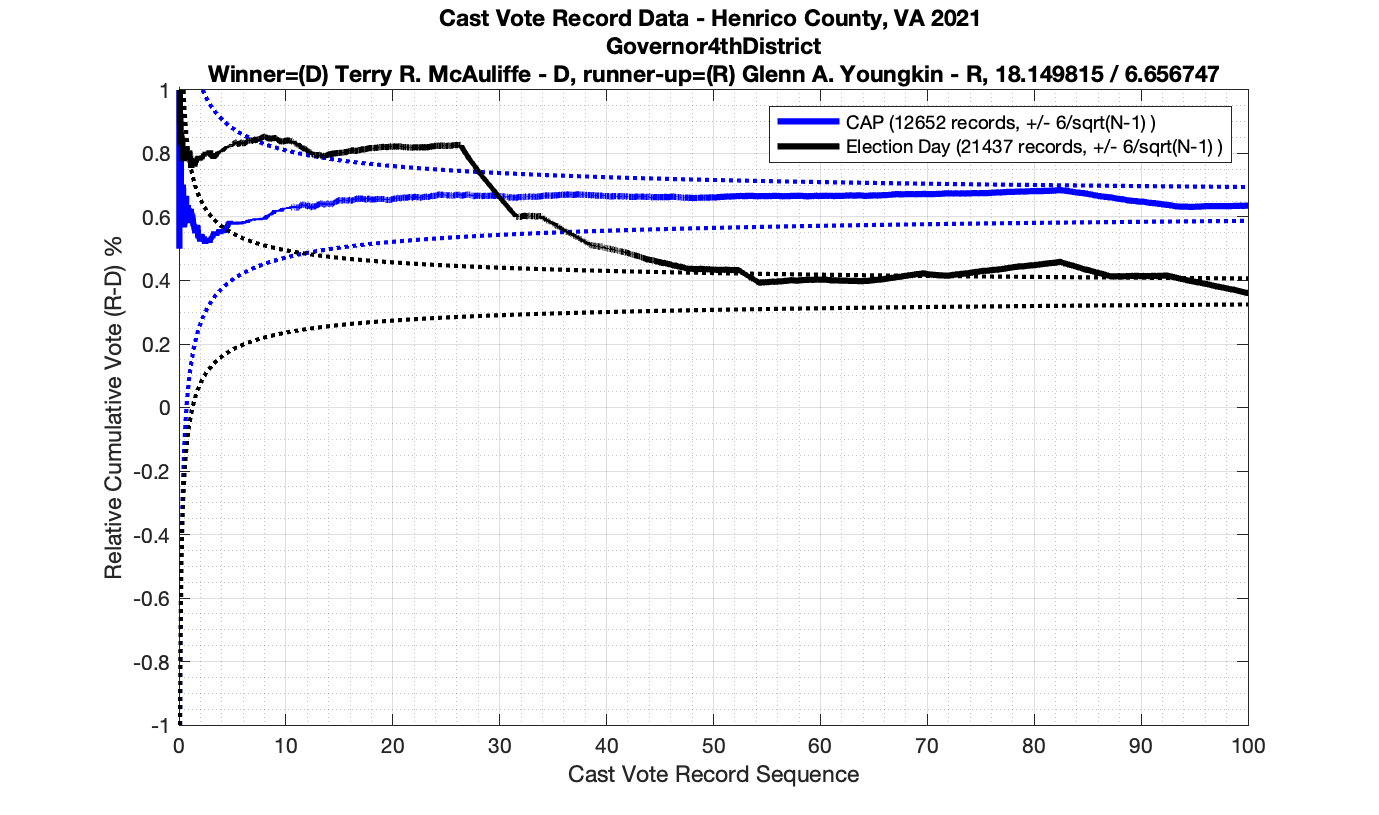
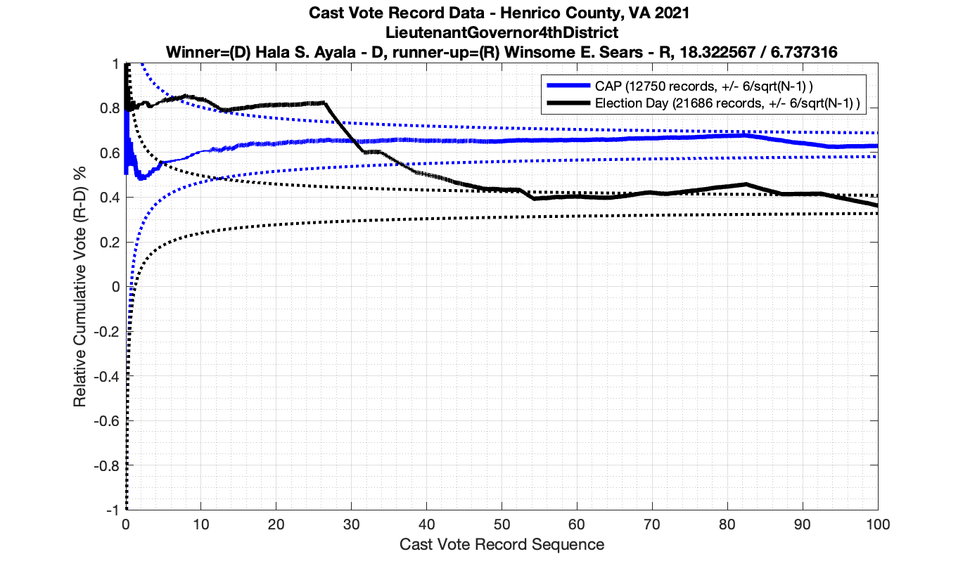
Moving to the Lt. Governors race we see an interesting phenomenon where where Ayala received a sudden 100 consecutive votes a little over midway through the counting process. Now granted, this was a landslide district for Ayala, but this still equates to a .92^100 = 0.000239 or 0.0239% chance of occurrence.
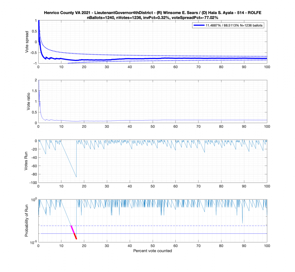
And here’s another large block of contiguous Ayala ballots equating to about .89^84 = 0.00005607 or 0.0056% chance of occurrence.
Tests for Differential Invalidation (added 2022-09-19):
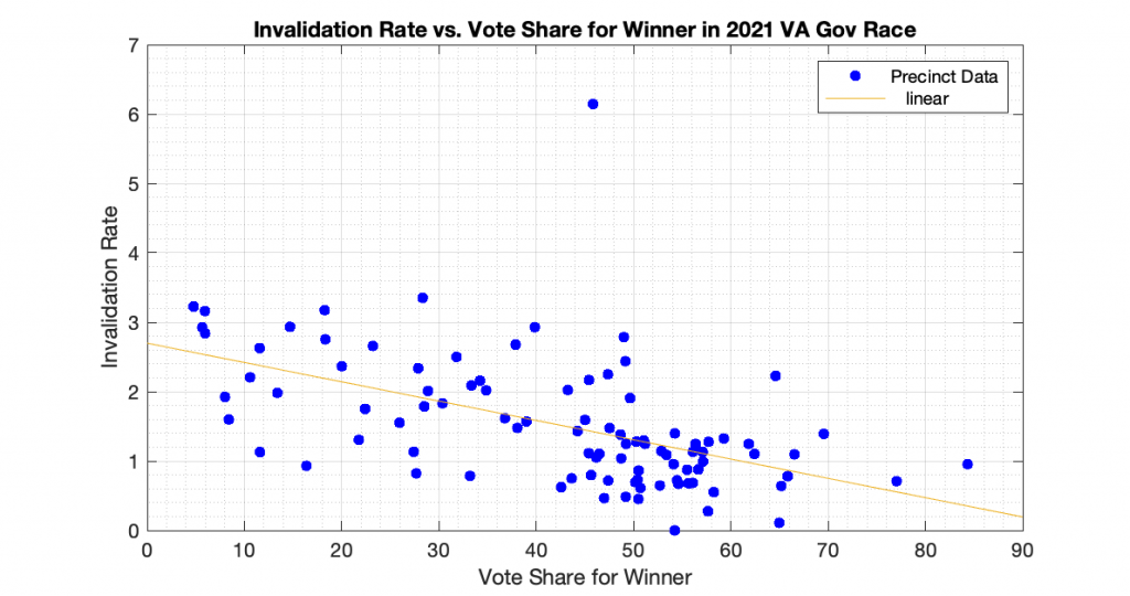
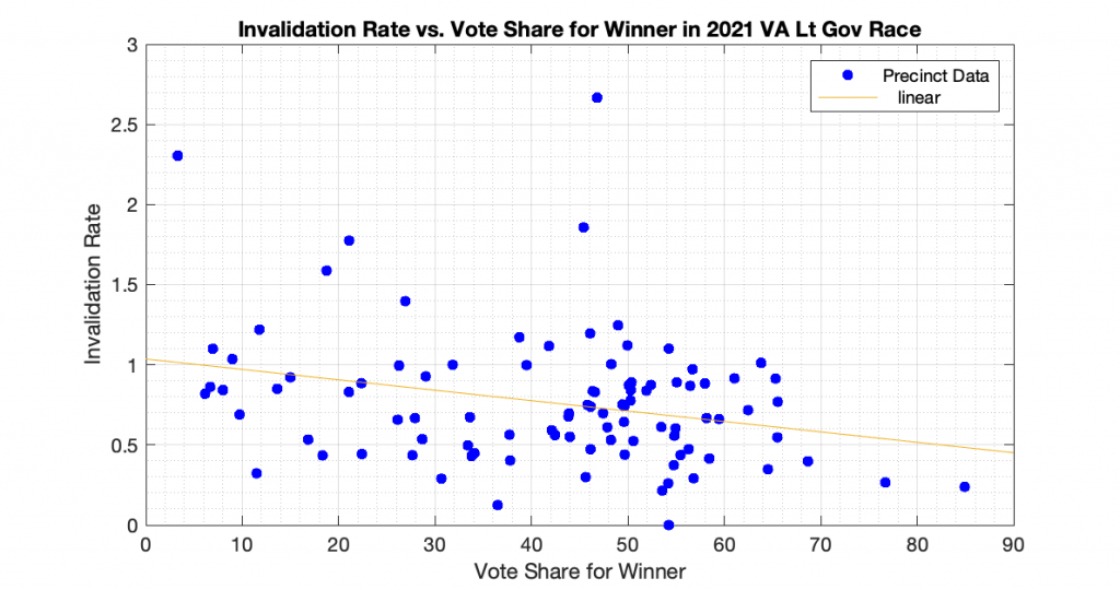
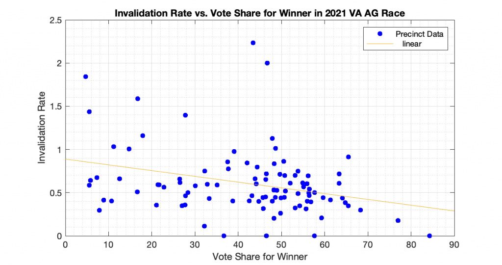
“Differential invalidation” takes place when the ballots of one candidate or position are invalidated at a higher rate than for other candidates or positions. With this dataset we know how many ballots were cast, and how many ballots had incomplete or invalid results (no recorded vote in the cvr, but the ballot record exists) for the 3 statewide races. In accordance with the techniques presented in [1] and [2], I computed the plots of the Invalidation Rate vs the Percent Vote Share for the Winner in an attempt to observe if there looks to be any evidence of Differential Invalidation ([1], ch 6). This is similar to the techniques presented in [2], which I used previously to produce my election fingerprint plots and analysis that plotted the 2D histograms of the vote share for the winner vs the turnout percentage.
The generated the invalidation rate plots for the Gov, Lt Gov and AG races statewide in VA 2021 are below. Each plot below is representing one of the statewide races, and each dot is representing the ballots from a specific precinct. The x axis is the percent vote share for the winner, and the y axis is computed as 100 – 100 * Nvotes / Nballots. All three show a small but statistically significant linear trend and evidence of differential invalidation. The linear regression trendlines have been computed and superimposed on the data points in each graph.
To echo the warning from [1]: a differential invalidation rate does not directly indicate any sort of fraud. It indicates an unfairness or inequality in the rate of incomplete or invalid ballots conditioned on candidate choice. While it could be caused by fraud, it could also be caused by confusing ballot layout, or socio-economic issues, etc.
[1] Forsberg, O.J. (2020). Understanding Elections through Statistics: Polling, Prediction, and Testing (1st ed.). Chapman and Hall/CRC. https://doi.org/10.1201/9781003019695
[2] Klimek, Peter & Yegorov, Yuri & Hanel, Rudolf & Thurner, Stefan. (2012). Statistical Detection of Systematic Election Irregularities. Proceedings of the National Academy of Sciences of the United States of America. 109. 16469-73. https://doi.org/10.1073/pnas.1210722109.
Update 2022-08-29 per observations by members of the Texas team I am working with, we’ve been able to figure out that (a) the vendor was simply concatenating data records from each machine and not sorting the CVR results and (b) how to mostly unwrap this affect on the data to produce much cleaner results. The results below are left up for historical reference.
For background information, please see my introduction to Cast Vote Records processing and theory here: Statistical Detection of Irregularities via Cast Vote Records. This entry will be specifically documenting the results from processing the Henrico County Virginia CVR data from the 2021 election.
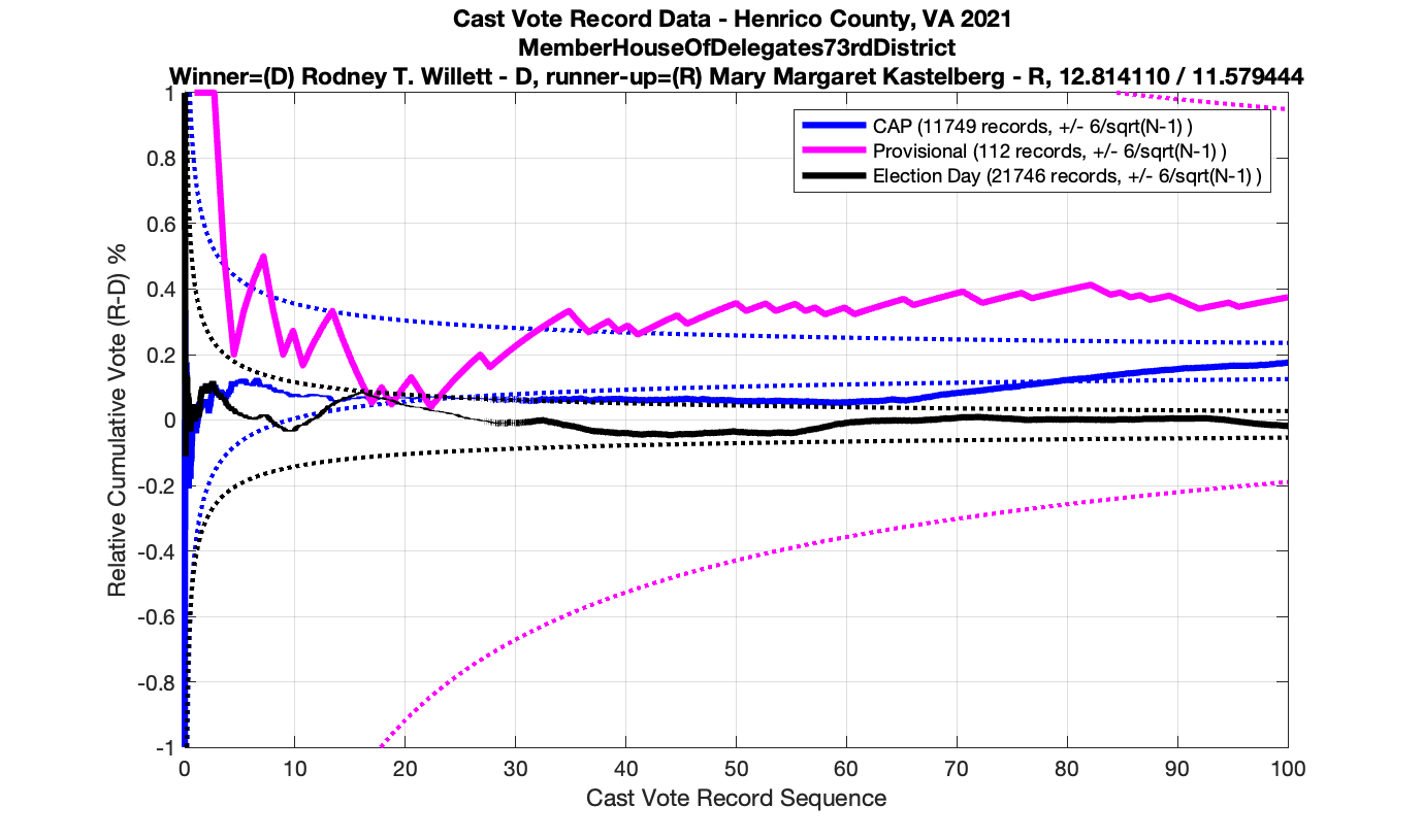
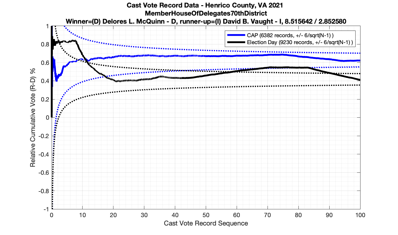
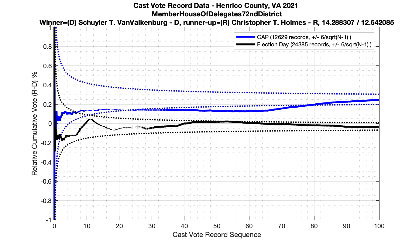
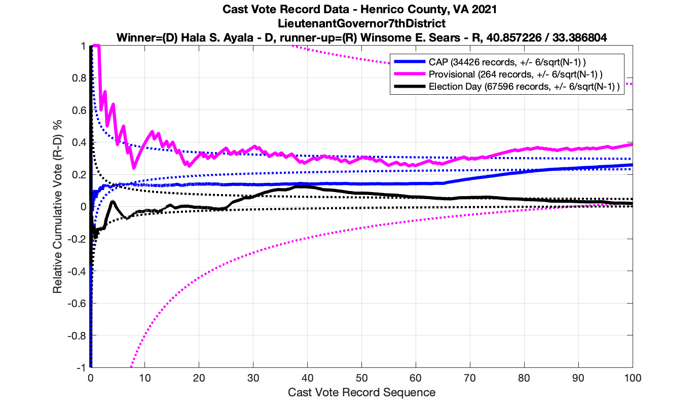
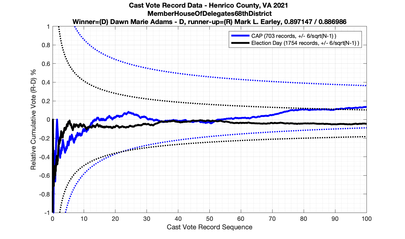
As in the results from the previous post, I expanded the theoretical error bounds out to 6/sqrt(N) instead of 3/sqrt(N) in order to give a little bit of extra “wiggle room” for small fluctuations.
However the Henrico dataset could only be broken up by CAP, Non-CAP or Provisional. So be aware that the CAP curves presented below contain a combination of both early-vote and mail-in ballots.
The good news is that I’ve at least found one race that seems to not have any issues with the CVR curves staying inside the error boundaries. MemberHouseOfDelegates68thDistrict did not have any parts of the curves that broke through the error boundaries.
The bad news … is pretty much everything else doesn’t. I cannot tell you why these curves have such differences from statistical expectation, just that they do. We must have further investigation and analysis of these races to determine root cause. I’ve presented all of the races that had sufficient number of ballots below (1000 minimum for the race a whole, and 100 ballot minimum for each ballot type).
There has been a good amount of commotion regarding cast vote records (CVRs) and their importance lately. I wanted to take a minute and try and help explain why these records are so important, and how they provide a tool for statistical inspection of election data. I also want to try and dispel any misconceptions as to what they can or can’t tell us.
I have been working with other local Virginians to try and get access to complete CVRs for about 6 months (at least) in order to do this type of analysis. However, we had not had much luck in obtaining real data (although we did get a partial set from PWC primaries but it lacked the time-sequencing information) to evaluate until after Jeff O’Donnell (a.k.a. the Lone Raccoon) and Walter Dougherity did a fantastic presentation at the Mike Lindell Moment of Truth Summit on CVRs and their statistical use. That presentation seems to have broken the data logjam, and was the impetus for writing this post.
Just like the Election Fingerprint analysis I was doing earlier that highlighted statistical anomalies in election data, this CVR analysis is a statistics based technique that can help inform us as to whether or not the election data appears consistent with expectations. It only uses the official results as provided by state or local election authorities and relies on standard statistical principles and properties. Nothing more. Nothing less.
What is a cast vote record?
A cast vote record is part of the official election records that need to be maintained in order for election systems to be auditable. (see: 52 USC 21081 , NIST CVR Standard, as well as the Virginia Voting Systems Certification Standards) They can have many different formats depending on equipment vendor, but they are effectively a record of each ballot as it was recorded by the equipment. Each row in a CVR data table should represent a single ballot being cast by a voter and contain, at minimum, the time (or sequence number) when the ballot was cast, the ballot type, and the result of each race. Other data might also be included such as which precinct and machine performed the scanning/recording of the ballot, etc. Note that “cast vote records” are sometimes also called “cast voter records”, “ballot reports” or a number of other different names depending on the publication or locality. I will continue to use the “cast vote record” language in this document for consistency.
Why should we care?
The reason these records are so important, is based on statistics and … unfortunately … involves some math to fully describe. But to make this easier, let’s try first to walk through a simple thought experiment. Let’s pretend that we have a weighted, or “trick” coin, that when flipped it will land heads 53% of the time and land tails 47% of the time. We’re going to continuously flip this coin thousands of times in a row and record our results. While we can’t predict exactly which way the coin will land on any given toss, we can expect that, on average, the coin will land with the aforementioned 53/47 split.
Now because each coin toss constitutes an independent and identically distributed (IID) probability function, we can expect this sequence to obey certain properties. If as we are making our tosses, we are computing the “real-time” statistics of the percentage of head/tails results, and more specifically if we plot the spread (or difference) of those percentage results as we proceed we will see that the spread has very large swings as we first begin to toss our coin, but very quickly the variability in the spread becomes stable as more and more tosses (data) are available for us to average over. Mathematically, the boundary on these swings is inversely proportional to the square root of how many tosses are performed. In the “Moment of Truth” video on CVRs linked above, Jeff and Walter refer to this as a “Cone of Probability”, and he generates his boundary curves experimentally. He is correct. It is a cone of probability as its really just a manifestation of well-known and well-understood Poisson Noise characteristic (for the math nerds reading this). In Jeff’s work he uses the ratio of votes between candidates, while I’m using the spread (or deviation) of the vote percentages. Both metrics are valid, but using the deviation has an easy closed-form boundary curve that we don’t need to generate experimentally.
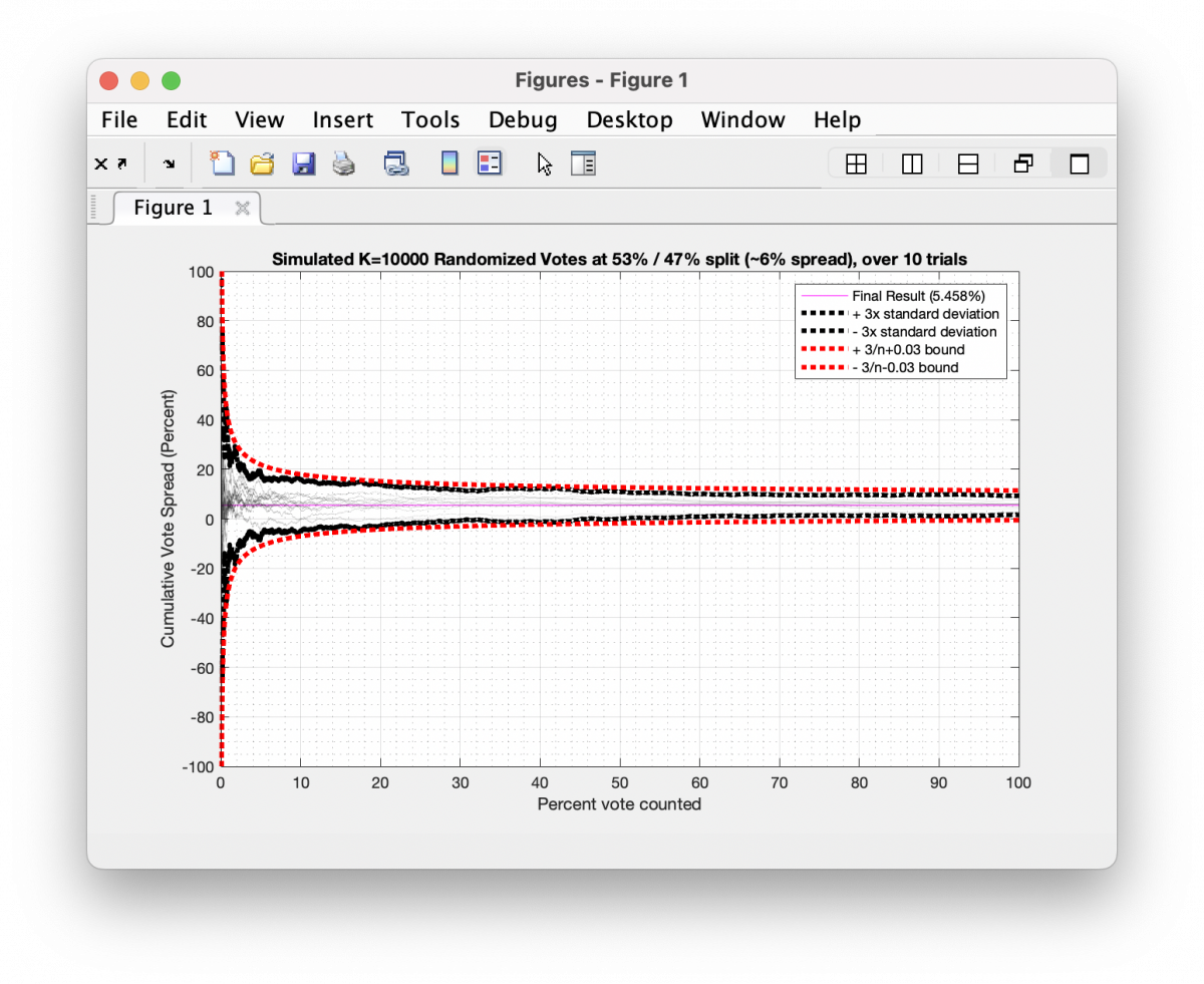
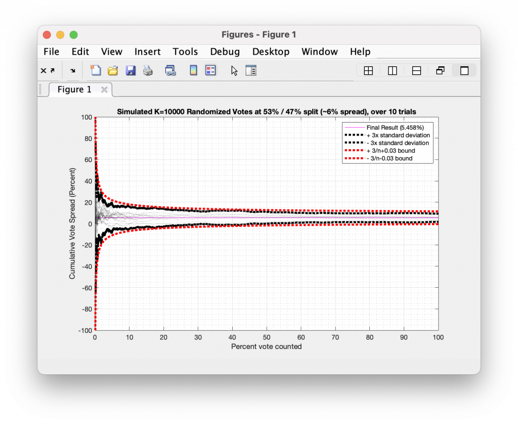
In the graphic below I have simulated 10 different trials of 10,000 tosses for a distribution that leans 53/47, which is equivalent to a 6% spread overall. Each trial had 10,000 random samples generated as either +1 or -1 values (a.k.a. a binary “Yes” or “No” vote) approximating the 53/47 split and I plotted the cumulative running spread of the results as each toss gets accumulated. The black dotted outline is the 95% confidence interval (or +/-3x the standard deviation) across the 10 trials for the Nth bin, and the red dotted outline is the 3/sqrt(n-1) analytical boundary.
So how does this apply to election data?
In a theoretically free and perfectly fair election we should see similar statistical behavior, where each coin toss is replaced with a ballot from an individual voter. In a perfect world we would have each vote be completely independent of every other vote in the sequence. In reality we have to deal with the fact that there can be small local regions of time in which perfectly legitimate correlations in the sequence of scanned ballots exist. Think of a local church who’s congregation is very uniform and they all go to the polls after Sunday mass. We would see a small trend in the data corresponding to this mass of similar thinking peoples going to the polls at the same time. But we wouldn’t expect there to be large, systematic patterns, or sharp discontinuities in the plotted results. A little bit of drift and variation is to be expected in dealing with real world election data, but persistent and distinct patterns would indicate a systemic issue.
Now we cannot isolate all of the variables in a real life example, but we should try as best as possible. To that effect, we should not mix different ballot types that are cast in different manners. We should keep our analysis focused within each sub-group of ballot type (mail-in, early-vote, day-of, etc). It is to the benefit of this analysis that the very nature of voting, and the procedures by which it occurs, is a very randomized process. Each sub-grouping has its own quasi-random process that we can consider.
While small groups (families, church groups) might travel to the in-person polls in correlated clusters, we would expect there to be fairly decent randomization of who shows up to in-person polls and when. The ordering of who stands in line before or after one another, how fast they check-in and fill out their ballot, etc, are all quasi-random processes.
Mail-in ballots have their own randomization as they depend on the timing of when individuals request, fill-out and mail their responses, as well as the logistics and mechanics of the postal service processes themselves providing a level of randomization as to the sequence of ballots being recorded. Like a dealer shuffling a deck of cards, the process of casting a mail-in vote provides an additional level of independence between samples.
No method is going to supply perfect theoretical independence from ballot to ballot in the sequence, but theres a general expectation that voting should at least be similar to an IID process.
Also … and I cannot stress this enough … while these techniques can supply indications of irregularities and discrepancies in elections data, they are not conclusive and must be coupled with in-depth investigations.
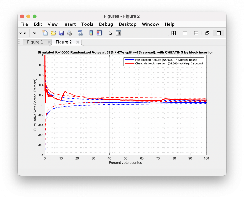
So going back to the simulation we generated above … what does a simulation look like when cheating occurs? Let’s take a very simple cheat from a random “elections” of 10,000 ballots, with votes being representative of either +1 (or “Yes”) or -1 (or “No”) as we did above. But lets also cheat by randomly selecting two different spots in the data stream to place blocks of 250 consecutive “Yes” results.
The image below shows the result of this process. The blue curve represents the true result, while the red curve represents the cheat. We see that at about 15% and 75% of the vote counted, our algorithm injected a block of “Yes” results, and the resulting cumulative curve breaks through the 3/sqrt(N-1) boundary. Now, not every instance or type of cheat will break through this boundary, and there may be real events that might explain such behavior. But looking for CVR curves that break our statistical expectations is a good way to flag items that need further investigation.
Computing the probability of a ballot run:
Section added on 2022-09-18
We can also a bit more rigor to the statistics outlier detection by computing the probability of the length of observed runs (e.g. how many “heads” did we get in a row?) occurring as we move through the sequential entries. We can compute this probability for K consecutive draws using the rules of statistical independence, which is P([a,a,a,a]) = P(a) x P(a) x P(a) x P(a) = P(a)^4. Therefore the probability of getting 4 “heads” in a row with a hypothetical 53/47 weighted coin would be .53^4 = 0.0789.
Starting with my updated analysis of 2021 Henrico County VA, I’ve started adding this computation to my plots. I have not yet re-run the Texas data below with this new addition, but will do so soon and update this page accordingly.
Real Examples
UPDATE 2022-09-18:
I have finally gotten my hands on some data for 2020 in VA. I will be working to analyze that data and will report what I find as soon as I can, but as we are approaching the start of early voting for 2022, my hands are pretty full at the moment so it might take me some time to complete that processing.
As noted in my updates to the Henrico County 2021 VA data, and in my section on computing the probability of given runs above, the Texas team noticed that we could further break apart the Travis county data into subgroups by USB stick. I will update my results below as soon as I get the time to do so.
So I haven’t gotten complete cast vote records from VA yet (… which is a whole other set of issues …), but I have gotten my Cheeto stained fingers on some data from the Travis County Texas 2020 race.
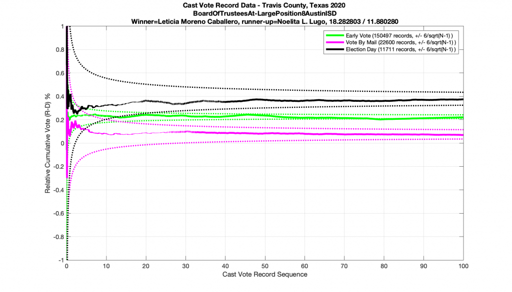
So let us first take a look at an example of a real race where everything seems to be obeying the rules as set out above. I’ve doubled my error bars from 3x to 6x of the inverse square standard (discussed above) in order to handle the quasi-IID nature of the data and give some extra margin for small fluctuating correlations.
The plot below shows the Travis County Texas 2020 BoardOfTrusteesAt_LargePosition8AustinISD race, as processed by the tabulation system and stratified by ballot type. We can see that all three ballot types start off with large variances in the computed result but very quickly coalesce and approach their final values. This is exactly what we would expect to see.
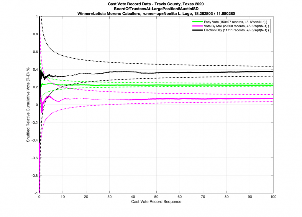
Now if I randomly shuffle the ordering of the ballots in this dataset and replot the results (below) I get a plot that looks unsurprisingly similar, which suggests that these election results were likely produced by a quasi-IID process.
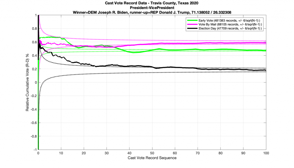
Next let’s take a look at a race that does NOT conform to the statistics we’ve laid out above. (… drum-roll please … as this the one everyone’s been waiting for). Immma just leave this right here and just simply point out that all 3 ballot type plots below in the Presidential race for 2020 go outside of the expected error bars. I also note the discrete stair step pattern in the early vote numbers. It’s entirely possible that there is a rational explanation for these deviations. I would sure like to hear it, especially since we have evidence from the exact same dataset of other races that completely followed the expected boundary conditions. So I don’t think this is an issue with a faulty dataset or other technical issues.
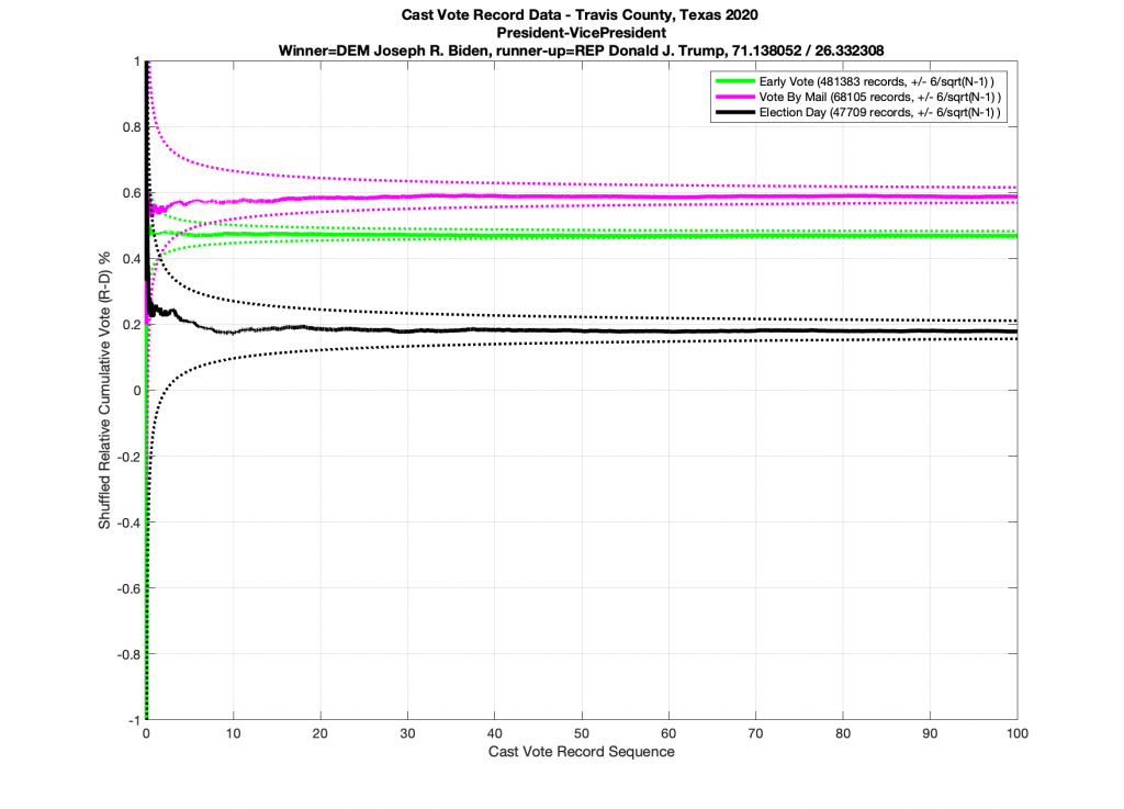
And just for completeness, when I artificially shuffle the data for the Presidential race, and force it to be randomized, I do in fact end up with results that conform to IID statistics (below).
I will again state that while these results are highly indicative that there were irregularities and discrepancies in the election data, they are not conclusive. A further investigation must take place, and records must be preserved, in order to discover the cause of the anomalies shown.
Running through each race that had at least 1000 ballots cast and automatically detecting which races busted the 6/sqrt(n-1) boundaries produces the following tabulated results. A 1 in the right hand column indicates that the CVR data for that particular race in Travis County has crossed the error bounds. A 0 in the right hand column indicates that all data stayed within the error bound limits.
[1] Forsberg, O.J. (2020). Understanding Elections through Statistics: Polling, Prediction, and Testing (1st ed.). Chapman and Hall/CRC. https://doi.org/10.1201/9781003019695
[2] Klimek, Peter & Yegorov, Yuri & Hanel, Rudolf & Thurner, Stefan. (2012). Statistical Detection of Systematic Election Irregularities. Proceedings of the National Academy of Sciences of the United States of America. 109. 16469-73. https://doi.org/10.1073/pnas.1210722109.