Update (2023-12-14 12:00:00 EST) : Special thank you to Rick Michael of the Chesterfield Electoral board for checking their records on issues #1 and #2 below. There were 3 x Issue #1 records and 9 x Issue #2 records identified in Chesterfield County.
According to Rick, the records in question were populated and visible when looking via the electronic VERIS (the states election database) login available to the Registrar. The 3 x Issue #1 records can be found and are Active records in the electronic system, and the 9 x Issue #2 records had an update that moved the records from Inactive to Active that were not reflected in the data supplied to us.
That implies that the data that we purchased (for approximately $12,000) directly from the department of elections is inaccurate and incomplete. Our initial purchase and download of the June 30 Registered Voter List (RVL) database does not show the registrants identified in Issue #1, even though the Registrar can see them in their electronic terminal. And our Monthly Update Subscription (MUS) we receive is missing the updates showing the registrant records identified in Issue #2 being moved from Inactive to Active status.
The department of elections is required by federal law (NVRA, HAVA) to keep and maintain accurate election records AND to make those records accessible for inspection and verification, and for use by candidates and political parties. Additionally, we have paid (twice!) for this data; once as taxpayers, and once again as a 501c3 entity. If the data we, and other campaigns and candidates are receiving is not representative of the actual records in the database, incomplete and inaccurate … that needs to be addressed and fixed.
Summary:
Issue #1: There are 99 records of ballots cast, according to the VA Department of Elections (ELECT) Daily Absentee List (DAL) data file that do not have corresponding voter ID listed in Registered Voter List (RVL) data.
Issue #2: There are 380 records of ballots cast in the DAL where the corresponding RVL record has been listed as “Inactive” since June-30-2023 and no modification to the RVL record has taken place.
Issue #3: There are 18 records of ballots cast in the DAL where the corresponding RVL record is listed as “Inactive” as of Dec-01-2023, but there has been previous modifications to the RVL record since June-30-2023.
We are currently reaching out in attempts to contact the VA AG’s office and to provide them the details of this analysis in order to have these anomalies further investigated.
Data files utilized for this analysis:
Our 501c3 EPEC purchased and downloaded the full statewide VA RVL on June-30-2023 from ELECT. We additionally purchased the Monthly Update Service (MUS) package from ELECT, where on the 1st of each month we are provided a list of all of the changes that have occurred to the RVL in the previous month. By applying these changes to our baseline data file, we are able to update our copy of the RVL to reflect the latest state as per ELECT. We can also create a cumulative record of all entries associated with a particular voter ID by simply concatenating all of these datafiles.
Additionally, during the VA 2023 General Election, we purchased access to the Daily Absentee List (DAL) file generated by ELECT that documents all of the transactions associated with early mail-in or in-person voting during the 45 day early voting period. The DAL file we utilized for this analysis was downloaded from ELECT on Nov-13-2023 at 6am EST.
Identification of ballots cast via the DAL file can be performed by checking for rows of the DAL data table that have the APP_STATUS field set to “Approved” and have the BALLOT_STATUS field set to any of the following: “Marked” | “Pre-Processed” | “On Machine” | “FWAB” | “Provisional”.
Once cast ballots are identified in the DAL, the Voter Identification Number can be used to lookup all of the corresponding records in our cumulative RVL data. The data issues summarized above can be directly observed using this process. Due to VA law, we cannot publish the full specific records here in this blog but have summarized, captured and described our process and results.
For Issue #1: If there does not exist a corresponding registration record for cast ballots, then the voter should not have been able to have their mail-in ballot approved or issued, or been able to check-in to an early voting precinct to vote on-machine. If the voter record actually does exists, then why is it not reflected in the data that we purchased from ELECT. Note that all provisional and Same Day Registration (SDR) ballots were required to be entered into the states database (“VERIS”) by the Friday after the election (Fri Nov-10-2023). We specifically waited until we received the Dec-01-2023 MUS data update from ELECT to attempt to perform this or similar analysis in order to ensure that we would not be missing any last minute registrations or RVL updates.
For Issue #2: There are 380 records of ballots being cast in the DAL where the baseline June-30-2023 RVL data file shows the registrant as inactive, and there has been no modifications or adjustments to the record presented in the MUS data files. Therefore these registrants should still have been listed as “Inactive” during the early voting period which started in September through Election Day (Nov 7).
For issue #3: There are 18 records that show the cast ballot is from a registrant that is currently listed as “Inactive” but there has been adjustments to the registration record over the last 6 months. An example of such is below. Note that I have captured the MUS data file generation dates in the 5th column to note when the file was generated and received by us.
In the example given below, the first invalidation operation on the registration record appears in the MUS file dated Sep-01, with the earliest transaction date listed as Aug-29-2023. The ballot application was not received until Sept 26 according to the DAL, so the application should never have been approved or the ballot issued as the registrant status should have been “Invalid” according to the states own data.
(Also … yes … I know there is a typo in the spelling of “APP_RECIEPT_DATE” in the tables below … but this is the data as it comes from ELECT).
APP_RECIEPT_DATE
APP_STATUS
BALLOT_RECEIPT_DATE
BALLOT_STATUS
“2023-09-26 00:00:00”
Approved
“2023-10-19 00:00:00”
Pre-Processed
Example Extract of a DAL data record for a mail-in ballot cast during early voting.
TRANSACTIONDATE
TRANSACTIONTIME
Trans_Type
NVRAReasonCode
File Source
30-June-2023
12:12:00
BASELINE
BASELINE
Baseline RVL
28-Jul-2023
09:34:03
MODIFY
Change Out
MUS 08/01/2023
28-Jul-2023
09:34:04
MODIFY
Address Change
MUS 08/01/2023
28-Jul-2023
09:34:04
MODIFY
Change In
MUS 09/01/2023
28-Jul-2023
09:34:03
MODIFY
Change Out
MUS 09/01/2023
28-Jul-2023
09:34:04
MODIFY
Address Change
MUS 09/01/2023
28-Jul-2023
09:34:04
MODIFY
Change In
MUS 09/01/2023
29-Aug-2023
11:55:49
MODIFY
Inactivate
MUS 09/01/2023
29-Aug-2023
11:55:49
MODIFY
Inactivate
MUS 10/01/2023
Extract of RVL Cumulative Data Records for Voter ID in above DAL entry
BLUF: The number of detected exact (Full Name + DOB) “clone” registration records in the VA Registered Voter List (RVL) file has decreased overall from 2022-11-23 to 2023-07-01, however there are additional new clones still being added to the database.
There has been a concentrated effort by various election integrity groups and public officials around the state of VA to clean up the voter rolls. Specifically the VA Department of Elections (“ELECT”) made a concerted effort in early 2023 to remove and clean up a large number (~19,000) of deceased voters and other errant records. The data below shows that these efforts have made an impact on the number of exact “clones” identified in the database, but that there is still more work to do.
BACKGROUND: This is a continuation of exploratory analysis on the existence of “cloned” records in the VA Registered Voter List. Please see previous posts here, here, here and here for background information.
As a reminder and for the purposes of this analysis, a potential “cloned” record is defined as a record in the VA Registered Voter List (RVL) where the Full Name (First + Middle + Last + Suffix) and full Date of Birth (mm/dd/yyyy) exactly matches another record but they have different Voter Identification Numbers. In my previous analyses I was focusing on the Active registration records that had been identified as clones, but even if a cloned record is marked as Inactive in the database, it still holds the potential to be voted as any interaction with the voter immediately moves the registration from Inactive to Active. Therefore the analysis below includes both Active and Inactive records.
It is important to note and emphasize that this analysis is onlyspecifically focusing on exact clones, and not any other of the number of potential errors that could be represented in a voter database. There are a couple of reasons for this narrow focus:
The detection of exact clones in the database requires no additional data correlations and can operate directly on the data provided from ELECT. It is easily defined and scriptable, and can be replicated by other researchers and public officials for verification.
Due to item (1), the identification of exact clones is a good candidate to track over time as a proxy indicator for issues with the database.
There are some rather interesting non-random distribution patterns of the already observed cloned records that I have previously discussed here, and I am interested in observing and understanding the cause of these distribution shapes.
DETAILS: As we now have collected multiple statewide voter registration lists, I was curious as to how the numbers of detected cloned registrant records have changed over time, specifically with respect to the REGISTRATION_DATE field that is reported in each record.
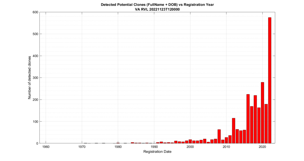
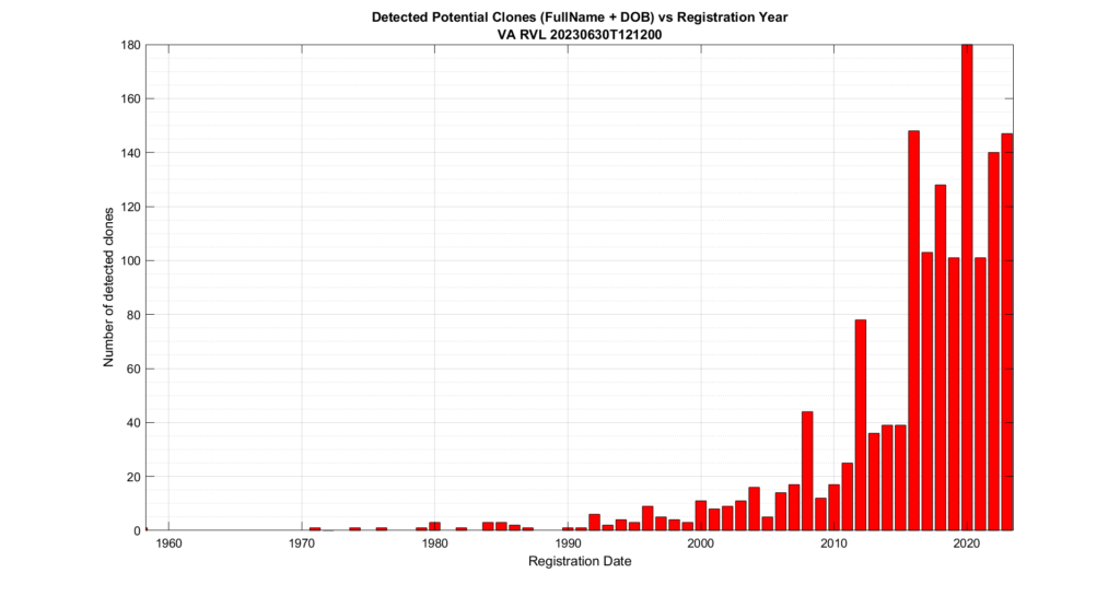
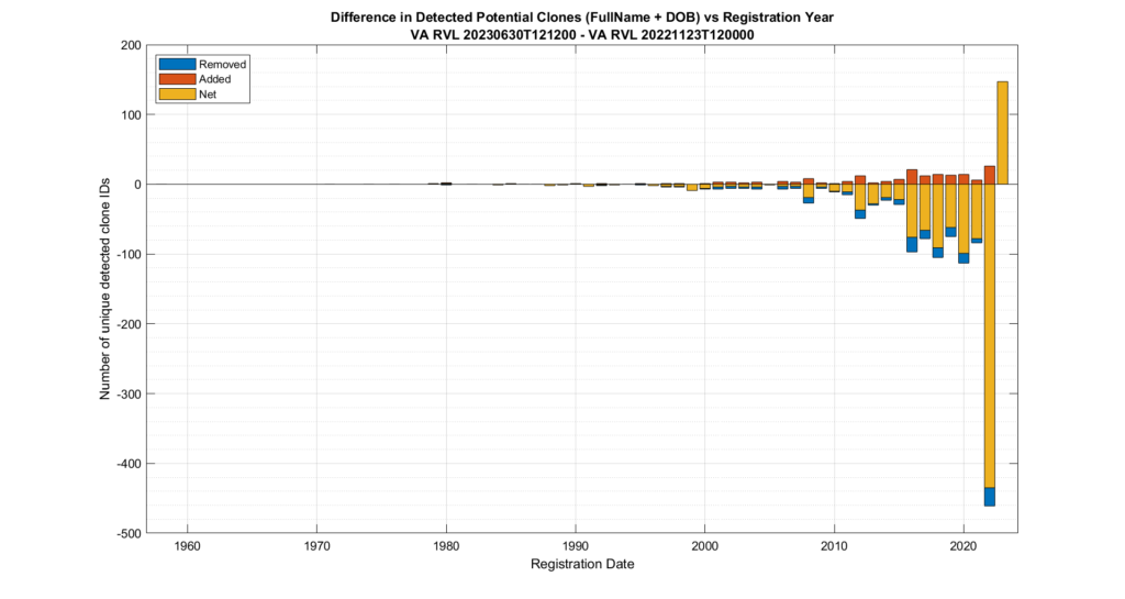
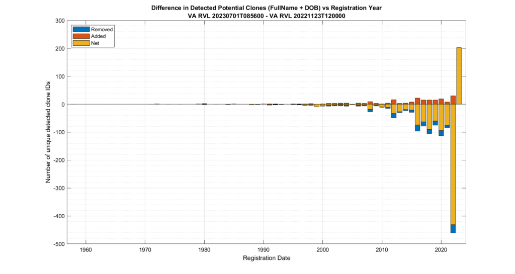
In Figure 1 below I’ve plotted the number of identified cloned records in the 2022-11-23 RVL stratified by registration date year. Figure 2 is the same plot from the 2023-06-30 RVL file we recently purchased. Figure 3 shows the number of additions, removals and net change in the number of identified cloned records in each date bin between these two datasets, based on the unique set of cloned Voter ID Numbers that fall within each bin.
Figure 1 Distribution of identified cloned records with respect to registration date in the 2022-11-23 Registered Voter List purchased from VA Department of Elections. The total number of identified (First + Middle + Last + Suffix + DOB) clones in the dataset was 2,445.Figure 2 Distribution of identified cloned records with respect to registration date in the 2023-06-30 Registered Voter List purchased from VA Department of Elections. The total number of identified (First + Middle + Last + Suffix + DOB) clones in the dataset was 1,485.Figure 3 Differences between the 2023-06-30 and 2022-11-23 RVL datasets.
The total number of identified clones in the 2022-11-23 dataset was 2,445. The total number of identified clones in the 2023-06-30 was 1,485. We can see in Figure 3 that while there has been an overall reduction of 960 in the number of cloned records (which is good!), there are still new clones being added to the voter registration database, even as previously identified clones have been removed. This suggests that there is an ongoing process(es) or mechanism(s) that is continuously adding cloned records to the voter list database.
It is not readily apparent as to what causes the added cloned records. It could be any number of technology issues, such as a poor input verification or coding practices, or related to human error and poor procedures and/or training, or a mixture of issues.
The two full datasets above (2022-11-23 and 2023-06-30) were purchased directly from the department of elections. The lists were parsed, standardized and normalized for string case, known typos, whitespace and punctuation issues, but otherwise the raw data entries were unadjusted.
We also purchased the Monthly Update Subscription (MUS) from ELECT at the time that we ordered the 2023-06-30 RVL. The MUS is generated on a monthly basis and captures the changes to the voter list over the prior month. We received the 2022-07-01 MUS, and applied the changes within it to the full 2023-06-30 RVL that we had received the day before. As the MUS contains all the changes over the previous month, and we had purchased our full dataset the prior day, we did not expect there to be many adjustments required, but there were a few. Applying the MUS to the 2023-06-30 dataset resulted in the generation of an updated 2023-07-01 dataset.
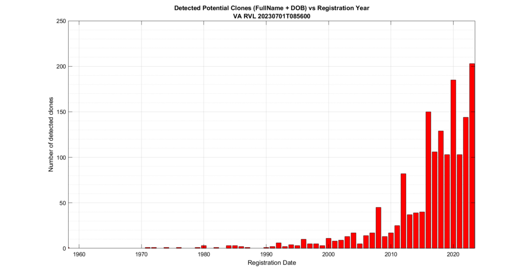
For completeness, the same plots that were generated above for the directly purchased data is repeated below for the updated RVL dataset. Figure 4 plots the number of identified cloned records in the 2023-07-01 RVL stratified by registration date year, and Figure 5 shows the differences with the 2022-06-23 dataset.
Figure 4 Distribution of identified cloned records with respect to registration date in the 2023-07-01 Registered Voter List generated from the purchased 2023-06-30 RVL and 2023-07-01 MUS files. The total number of identified (First + Middle + Last + Suffix + DOB) clones in the dataset was 1,575. Figure 5 Differences between the 2023-07-01 and 2022-11-23 RVL datasets.
One thing that I find interesting is the difference in detected cloned entries between the purchased 2023-06-30 dataset and the 2023-07-01 dataset after the MUS entries have been applied. This is presented in Figure 6 below. We see that the application of the MUS did not remove any clones, but 90 were added. I’m not sure what this means yet, as we only have a single MUS file and it was generated so close to our full download. We will monitor and see how this progresses as we continue to receive the MUS files throughout the 2023 election cycle.
One thing that I have been asked about repeatedly is if there is any sort of patterns in the assignment of voter ID numbers in the VA data. Specifically, I’ve been asked repeatedly if I’ve found any similar pattern to what AuditNY has found in the NY data. It’s not something that I have looked at in depth previously due mostly to lack of time, and because VA is setup very differently than NY, so a direct comparison or attempt to replicate the AuditNY findings in VA isn’t as straightforward as one would hope.
The NY data uses a different Voter ID number for counties vs at the state level, which is the “Rosetta Stone” that was needed for the NY team to understand the algorithms that were used to assign voter ID numbers, and in turn discover some very (ahem) “interesting” patterns in the data. VA doesn’t have such a system and only uses a single voter ID number throughout the state and local jurisdictions.
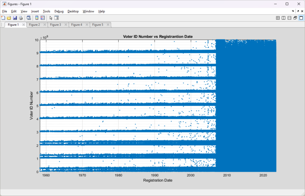
Well … while my other machine is busy crunching on the string distance computations, I figured I’d take a crack at looking at the distribution of the Voter ID numbers in the VA Registered Voter List (RVL) and just see what I find.
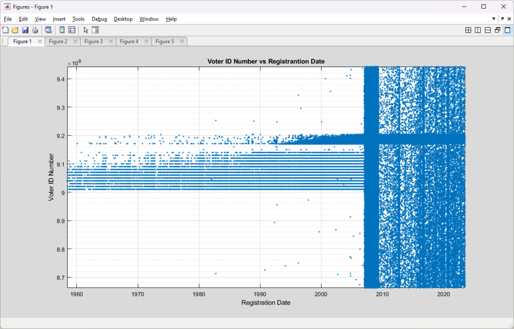
To start with, here is a simple scatter plot of the Voter ID numbers vs the Registration date for each record in the 2023-07-01 RVL. From the zoomed out plot it is readily apparent that there must have been a change in the algorithm that was used to assign voter identification numbers sometime around 2007, which coincides nicely with the introduction of the current Virginia Election and Registration Information System (VERIS) system.
From a high level, it appears that the previous assignment algorithm broke the universe of possible ID numbers up into discrete ranges and assigned IDs within those ranges, but favoring the bottom of each range. This would be a logical explanation for the banded structure we see pre-2007. The new assignment algorithm post-2007 looks to be using a much more randomized approach. Nothing strange about that. As computing systems have gotten better and security has become more of a concern over the years there have been many systems that migrated to more randomized assignments of identification numbers.
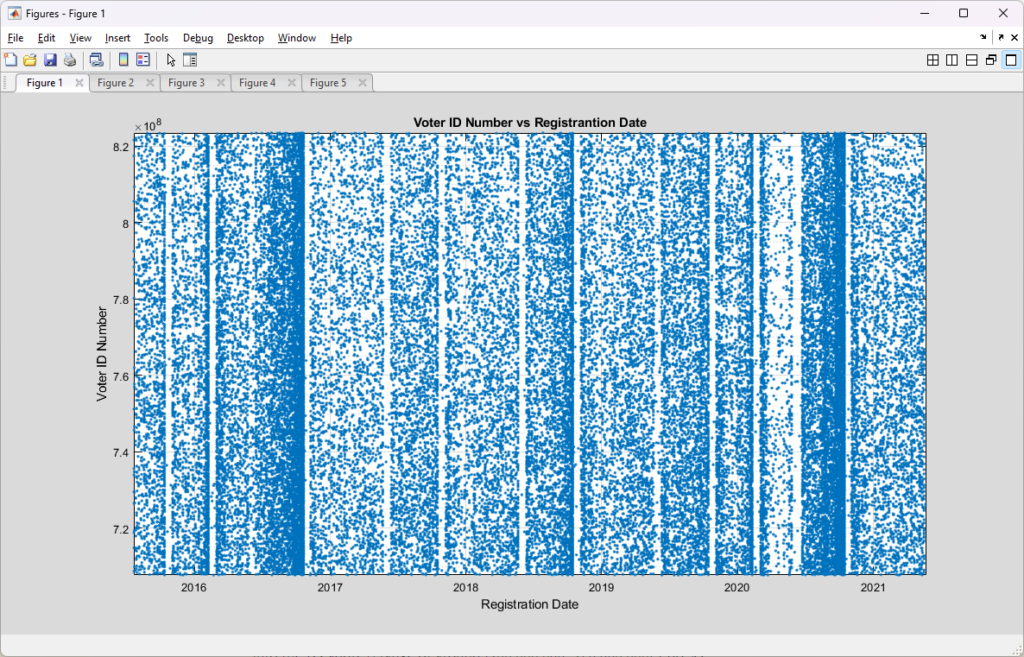
Looking at a zoomed in block of the post-2007 “randomized” ID assignments we can see some of the normal variability that we would expect to see in the election cycles. We see that we have a high density of new assignments around November of 2016 and 2020, with a low density section of assignments correlated to the COVID-19 lockdowns. There are short periods where it looks like there were lulls in the assignment of voter ID’s, these are perhaps due to holidays or maintenance periods, or related to the legal requirements to “freeze” the voter rolls 30 days before any election (primaries, runoffs, etc). Note that VA now has same day voter registration as of the laws passed by the previous democratic super-majority that went into affect in 2022, so going forward we would likely see these “blackout periods” be significantly reduced.
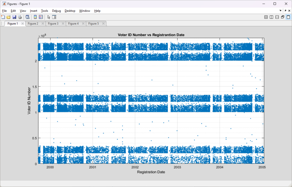
We can see more clearly the banded assignment structure of the pre-2007 entries by zooming in on a smaller section of the plot, as shown below. It’s harder to make out in this banded structure, but we still see similar patterns of density changes presumably due to the natural election cycles, holidays, maintenance periods, legally required registration lockouts periods, etc. We can also see the “bucketing” of ID numbers into distinct bands, with the bias of numbers filling the lower section of each band.
All of that looks unremarkable and seems to make sense to me … however … if we zoom into the Voter ID address range of around [900,000,000 to 920,000,000] we do see something that catches my curiosity. We see the existence of the same banded structure as above between 900,000,000 and 915,000,000 AND pre-2007, but there is another band of assignments super-imposed on the entire date range of the RVL. This band does not seem to be affected by the introduction of the VERIS system (presumably), which is very interesting. There is also what looks like to be a vertical high-density band between 2007 and 2010 that extends along the entire vertical axis, but we only see it once we zoom in to the VERIS transition period.
The horizontal band that extends across all date ranges only exists in the [~915,000,000 to ~920,000,000] ID range. It trails off in density pre ~1993, but it exists throughout the full registration date range. I will note that the “Motor Voter” National Voter Registration Act (NVRA) was implemented in 1993, so perhaps these are a reserved universe block for DMV (or other externally provided) registrations? (That’s a guess, but an educated one.)
A plausible explanation I can imagine for the distinct high density band between 2007-2010 is that this might be related to how the VERIS system was implemented and brought into service, and there was some sort of update around 2010 that made correction to its internal algorithms. (But that is just a guess.) That still wouldn’t entirely explain the huge change in the density of new registrants added to the rolls.
Another, or additional, explanation might be that when VERIS came online there were a number of registrants that had their Voter ID number regenerated and/or their registration date field updated as part of the rollout of the new VERIS software. Meaning that while VERIS was coming online and handling the normal amount of new real registrations, it was also moving/updating a large number of historic registrations, which would account for the higher density as VERIS became the system of record. That seems to be a poor systems administration and design choice, in my opinion, as it makes inaccurate those moved registrant records by giving them a false registration date. However, if that was the case, and VERIS was resetting registration dates as it ingested voter records into its databases, why do we see any records with pre-2007 registration dates at all? (This is again, merely an educated guess on my part, so take with a grain of salt.)
Incorporating the identification of cloned registrations
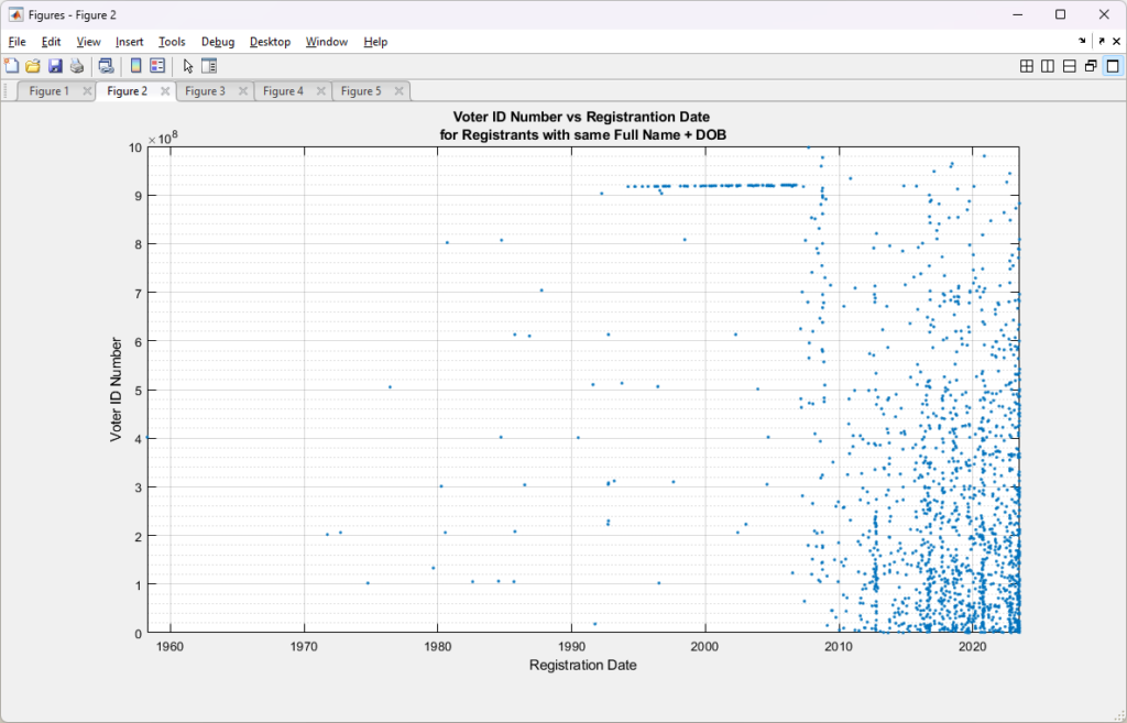
In attempting to incorporate some of my early results on the most recent RVL data doing duplicate record identification (technically they are “cloned” records, as “duplicates” would have the same voter ID numbers. This was pointed out to me a few days ago.) on this dataset, I did a scatter plot of only those records that had an identified exact match of (FullName +DOB) to other records in the dataset, but with unique Voter ID numbers. The scatter plot of those records is shown below, and we can see that there is a distinct ~horizontal cluster of records that aligns with the 915M – 920M ID band and pre-2007. In the post-2007 block we see the cloned records do not seem to be totally randomly distributed, but have a bias towards the lower right of the graph.
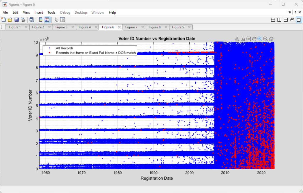
Superimposing the two plots produces the following, with the red indicating the records with identified Full Name + DOB string matches.
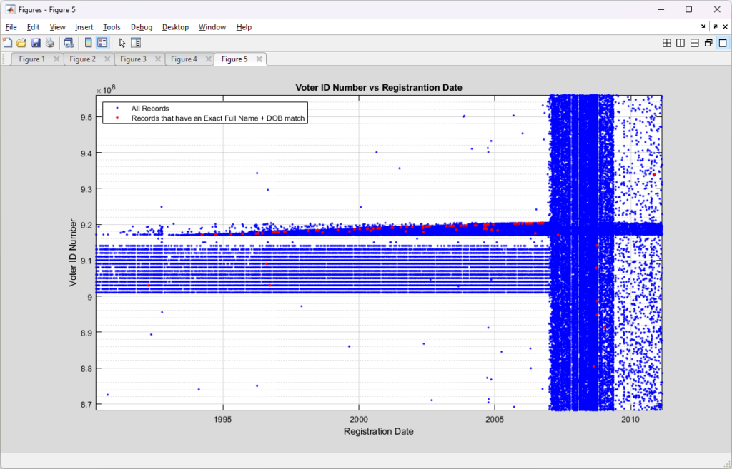
Zooming in to take a closer look at the 915M-920M band again, gives the following:
It is curious that there seems to be an alignment of the exact Full Name + DOB matching records with the 915M-920M, pre-2007 ID band. Post-2007 the exact cloned matches have a less structured distribution throughout the data, but they do seem to cluster around the lower right.
If the cloned records were simply due to random data entry errors, etc. I would expect to see sporadic red datapoints distributed “salt-n-pepper” style throughout the entirety of the area covered by the blue data. There might be some argument to be made for there being a bias of more of the red data points to the right side of the plot, as officials have not yet had time to “catch” or “clean-up” erroneous entries, but there is little reason to have linear features, or to have a bias for lower ID numbers in the vertical axis.
I am continuing to investigate this data, but as of right now all I can tell you is that … yes, there does seem to be interesting patterns in the way Voter IDs are assigned in VA, especially with records that have already been found and flagged to be problematic (clones).
Below are the preliminary results from performing exact (string distance of 0) duplicate record checks on the 2023-07-01 VA Registered Voter List information. Note that these are the numbers of ordered matches discovered, not the number of individual unique registrants. Each count represents two different registration records, with unique voter IDs, that match the given criteria. Match pairs are directional, in that a pair (A,B) is counted separately from the pair (B, A). Matches are grouped into this table according to the LOCALITY_NAME of the first element of the identified pair. Some pairs can have different locality information, except for in the strictest case (3rd column), so a match might be counted in one locality while its mirror is counted in the other.
The first data column of the table below is equivalent to the criteria used by the MOU between the VA Department of Elections (ELECT) and the Department of Motor Vehicles (DMV), as discussed and documented in a previous post. There were 5,290 matches for this criteria across the state.
The second data column below is based on a match of the registrants Full Name and Day+Month+Year of birth information, but NOT the registrants listed address information. There were 1,200 matches for this criteria across the state.
The third data column is the strictest match criteria and includes the Gender and Address of the registrant. There were 208 matches for this criteria across the state.
I am only considering Active registrations in the table below. I previously computed similar statistics using the previous purchased 2022-11-23 RVL, I have not yet done a comparison of the two datasets, but will do so once I complete the string distance processing on this latest set.
Row Labels
Sum of Exact Same First+Last+Dob
Sum of Exact Same First+Middle+Last+Sfx+DOB
Sum of Exact Same First+Middle+Last+Sfx+Gender+Address+DOB
Previously I posted the computation of potential duplicate records based on string comparisons in the registered voter list. As a follow up to that article, I’ve compiled the statistics of the number of potential pairs for each locality in VA.
I tallied the number of registrant pairs with the reference match criteria defined by the MOU between ELECT and the DMV along with the two highest confidence (most stringent) match criteria that I computed. I also stratified the results by Active registrant records only or either Active or Inactive records. I also stratified by if the pairs crossed a locality boundary or not.
The table below is organized into the following computed columns, and has been sorted in decreasing order according to column 5.
Exactly matching First + Last + DOB, which is equivalent to the MOU between ELECT and DMV.
Exactly matching First + Middle + Last + Suffix + DOB
Exactly matching First + Middle + Last + Suffix + DOB + Gender + Street Address
The same as #1, but filtering for only ACTIVE voter records
The same as #2, but filtering for only ACTIVE voter records
The same as #3, but filtering for only ACTIVE voter records
The same as #1, but filtering for only pairs that cross a locality boundary.
The same as #2, but filtering for only pairs that cross a locality boundary.
The same as #3, but filtering for only pairs that cross a locality boundary.
The same as #4, but filtering for only pairs that cross a locality boundary.
The same as #5, but filtering for only pairs that cross a locality boundary.
The same as #6, but filtering for only pairs that cross a locality boundary.
1
2
3
4
5
6
7
8
9
10
11
12
LOCALITY_NAME
Num Registrant Records
Pct Same First Last Dob
Pct Same Full Name Dob
Pct Same Full Name Dob Address
Pct Same First Last Dob _ Active Only
Pct Same Full Name Dob _ Active Only
Pct Same Full Name Dob Address _ Active Only
Pct Same First Last Dob _ xLoc
Pct Same Full Name Dob _ xLoc
Pct Same Full Name Dob Address _ xLoc
Pct Same First Last Dob _ Active Only _ xLoc
Pct Same Full Name Dob _ Active Only _ xLoc
Pct Same Full Name Dob Address _ Active Only _ xLoc
I previously documented the utilization of the Hamming string distance measure to identify candidate pairs of duplicate registrants in voter lists. While a good first attempt at quantifying the numbers of potential duplicates in the voter rolls, using a hamming distance metric is less than ideal for reasons discussed below and in the previous article. I have since been able to update the processing functions to use a more complete Levenshtein distance (LD) metric, and made some improvements to parsers and other code utilities, etc., but otherwise the the analysis followed the same procedure, and is described below.
Using the 2022-11-23 Registered Voter List (RVL) and the 2023-01-26 Voter History List (VHL) purchased from the VA Department of Elections (ELECT) I wrote up an analysis script to check for potentially duplicated registrant records in the RVL and cross reference duplicate pairings with the VHL to identify potential duplicate votes. The details are summarized below.
Please note that I will not publish voter Personally Identifiable Information (PII) on this blog. I have substituted fictitious PII information for all examples given below, and cryptographically hashed all voter information in the downloadable results file. I will make available the detailed information to those that have the authorization to receive and process voter data upon request (contact us).
Summary of Results:
As a baseline, there were 6,464 records for STATUS=’Active’ registrants that adhered to the definition of a “duplicate” when Social Security Number (SSN) is not available, as defined by the MOU between DMV and ELECT (section 7.3) of having the same First Name + Last Name + Full Date of Birth (DOB). I’ve included a copy of the MOU between the VA DMV and ELECT at the end of this article for reference. It should be noted that most records held by DMV and ELECT have a SSN associated with them (or at least they should). SSN information is not distributed as part of the data purchased from ELECT, however, so this is the appropriate standard baseline for this work.
Upgrading our definition of a potential duplicate to [First + Middle + Last + Suffix + DOB] and using a LevenshteinDistance=0 drops the number of potential duplicates to 1,982, with each identified registrant in a pair having an exactly matching string result and unique voter ID numbers.
According to my derivations and simulations that are described in detail here, we should only expect to see an average of 11 (+/- 3) potential duplicate pairs (a.k.a. “collisions”) at a distance of 0. This is over two orders of magnitude different than what we observe in the compiled results. Such a discrepancy deserves further investigation and verification.
Allowing for a single string difference by setting LevenshteinDistance<=1 increases the pool of potential duplicates to 5,568. While this relaxation of the filter does allow us to find certain issues (described below) it also increases our chances of finding false positives as well. The LD metric results should not be viewed as a final determination, but as simply a useful tool to make an initial pass through the data and find candidate matches that still require further review, verification and validation.
Increasing to LevenshteinDistance<=2 brings the number of potential duplicates up to 32,610. When we increase to LD <= 3 we get an explosion of 183,130 potential duplicates.
Method:
For every entry in the latest RVL, I performed a string distance comparison, based on Levenshtein distance, between every possible pair of strings of (FIRST NAME + MIDDLE NAME + LAST NAME + SUFFIX + FULL DOB). For the ~6M different RVL entries, we therefore need to compute ~3.8 x 10^13 different string comparisons, and each string comparison can require upwards of 75 x 75 individual character comparisons, meaning the total number of character operations is on the order of 202.5 Quadrillion, not including logging and I/O.
A distance of 0 indicates the strings being compared are identical, a distance of 1 indicates that there a single character can be changed, inserted or removed that would convert one string into the other. A distance of 2 indicates that 2 modifications are required, etc.
Example: The string pair of “ALISHA” –> “ALISHIA” has an LD of 1, corresponding to the addition of an “I” before the final “A”.
I aggregated all of the Levenshtein distance pairings that were less than or equal to 3 characters different in order to identify potential (key word) duplicated registrants, and additionally for each pairing looked at the voter history information for each registrant in the pair to determine if there was a potential (again … key word) for multiple ballots to be cast by the same person in any given election. As we allow for more characters to be different, we potentially are including many more likely false positive matches, even if we are catching more true positives.
For example: At a distance of 4 the strings of “Dave Joseph Smith M 10/01/1981” and “Tony Joseph Smith M 10/01/1981” at the same address would produce a potential match, but so would “Davey Joseph Smith M 10/01/1981” and “David Josiph Smith M 10/02/1981”. The first pair is more likely to be a false positive due to twins, while the second is more likely to be due to typo’s, mistakes, or use of nicknames and might warrant further investigation. A much stronger potential match would be something like “David Josiph Smith M 10/01/1981” and “David Joseph Smith M 10/01/1981”, with a distance of 1 at the same address. In an attempt to limit false positives, I have clamped the distance checks to <= 3 in this analysis.
The Levenshtein distance measure is importantly able to identify potential insertions or deletions as well as character changes, which is an improvement over the Hamming distance measure. This is exampled by the following pairing: “David Joseph Smith M 10/01/1981” and “Dave Joseph Smith M 10/01/1981”. The change from “id” to “e” in the first name adds/subtracts a character making the rest of the characters in the remainder of the string shift position. A Levenshtein metric would correctly return a small distance of 2, whereas the hamming distance returns 27.
Note that with the official records obtained from ELECT, and in accordance with the laws of VA, I do not have access to the social security number or drivers license numbers for each registration record, which would help in identifying and discriminating potential duplicate errors vs things like twins, etc. I only have the first name, middle name, last name, suffix, month of birth, day of birth, year of birth, gender, and address information that I can work with. I can therefore only take things so far before someone else (with investigative authority and ability to access those other fields) would need to step in and confirm and validate these findings.
Results:
The summary totals are as follows, with detailed examples.
DMV_ELECT MOU Standard
LD <= 0
LD <= 1
LD <= 2
LD <= 3
Number of Potential Duplicate Registrant Pairs
7,586 (0.12%)
2,472 (0.04%)
6,620 (0.11%)
32,610 (0.53%)
183,130 (2.99%)
Number of Potential Duplicate Registrant Pairs (Active Only)
6,464 (0.11%)
1,982 (0.03%)
5,568 (0.10%)
28,884 (0.50%)
164,302 (2.85%)
Number of Potential Duplicate Ballots
6,362
112
3,576
37,028
236,254
Number of Potential Duplicate Ballots (Active Only)
6,228
110
3,542
36,434
232,394
Examples of Types of Issues Observed:
NOTE THE BELOW INFORMATION HAS HAD THE VOTER PERSONALLY IDENTIFIABLE INFORMATION (“PII”) FICTIONALIZED. WHILE THESE ARE BASED ON REAL DATA TO ILLUSTRATE THE DIFFERENT TYPES OF OBSERVATIONS, THEY DO NOT REPRESENT REAL VOTER INFORMATION.
Example #1: The following set of records has the exact match (distance = 0) of full name and full birthdate (including year), but different address and different voter ID numbers AND there was a vote cast from each of those unique voter ID’s in the 2020 General Election. While it’s remotely possible that two individuals share the exact same name, month, day and year of birth … it is probabilistically unlikely (see here), and should warrant further scrutiny.
Voter Record A:
AMY BETH McVOTER 12/05/1970 F 12345 CITIZEN CT
Voter Record B:
AMY BETH McVOTER 12/05/1970 F 5678 McPUBLIC DR
Example #2: This set of records has a single character different (distance of 1) in their first name, but middle name, last name, birthdate and address are identical AND both records are associated with votes that were cast in the 2020, 2021, and 2022 November General Elections. While it is possible that this is a pair of 23 year old twins (with same middle names) that live together, it at least bears looking into.
Voter Record A:
TAYLOR DAVID VOTER 02/16/2000 M 6543 OVERLOOK AVE NW
Voter Record B:
DAYLOR DAVID VOTER 02/16/2000 M 6543 OVERLOOK AVE NW
Example #3: This set of records has two characters different (distance of 2) in their birthdate, but name and address are identical AND the birth years are too close together for a child/parent relationship, AND both records are associated with votes that were cast in the 2020 and 2022 November General Elections.
Voter Record A:
REGINA DESEREE MACGUFFIN 02/05/1973 F 123 POPE AVE
Voter Record B:
REGINA DESEREE MACGUFFIN 03/07/1973 F 123 POPE AVE
Example #4: This set of records has again a single character different (distance of 1) in the first name (but not the first letter this time) and the last name, birthdate and address are identical. There were also multiple votes cast in the 2019 and 2022 November General from these registrants.
Voter Record A:
EDGARD JOHNSON 10/19/1981 M 5498 PAGELAND BLVD
Voter Record B:
EDUARD JOHNSON 10/19/1981 M 5498 PAGELAND BLVD
Example #5: This set of records has two characters different (distance of 2) in the first and middle names and the last name, birthdate, gender and address are identical. There were also multiple votes cast in the 2021 and 2022 November General from these registrants. Again it is possible that these records represent a set of twins given the information that ELECT provides.
Voter Record A:
ALANA JAVETTE THOMPSON 01/01/2003 F 123 CHARITY LN
Voter Record B:
ALAYA YAVETTE THOMPSON 01/01/2003 F 123 CHARITY LN
Example #6: The following set of records has the exact match (Distance = 0) of full name and full birthdate (including year), and same address but different voter ID numbers. There was no duplicated votes in the same election detected between the two ID numbers.
Voter Record A:
JAMES TIBERIUS KIRK 03/22/2223 M 1701 Enterprise Bridge
Voter Record B:
JAMES TIBERIUS KIRK 03/22/2223 M 1701 Enterprise Bridge
Example #7: The following set of records has the exact match (distance = 0) of full name and full birthdate (including year), same address but different gender and voter ID numbers. There was no duplicated votes in the same election detected between the two ID numbers.
Voter Record A:
MAXWELL QUAID CLINGER 11/03/2004 M 4077 MASH DR
Voter Record B:
MAXWELL QUAID CLINGER 11/03/2004 U 4077 MASH DR
Example #8: The following set of records has a single punctuation character different, with the same address but different voter ID numbers. There was no duplicated votes in the same election detected between the two ID numbers.
Voter Record A:
JOHN JACOB JINGLHIEMER-SCHMIDT 06/29/1997 M 12345 JACOBS RD
Voter Record B:
JOHN JACOB JINGLHIEMER SCHMIDT 06/29/1997 M 12345 JACOBS RD
Results Dataset:
A full version of the aggregated excel data is provided below, however all voter information (ID, first name, middle name, last name, dob, gender, address) have been removed and replaced by a one-way hash number, with randomized salt, based on the voter ID. The full file with specific voter information can be provided to parties authorized by ELECT to receive and process voter information, Election Officials, or Law Enforcement upon request.
The MOU between the VA Department of Elections (ELECT) and the VA Department of Motor Vehicles (DMV) is also provided below for reference. Section 7.3 defines the minimal standards for determining a match when no social security number is present.
Below I present the theory and derivation as to how I arrived at the expected value of 11 collisions (+/- 3) as mentioned in my posts discussing string distance analysis (here and here). I’ve tried to make the derivation below as digestible as possible, with accessible references, but it is admittedly still a very technical read. I think its important to “show my work” on the subject, though, and I present it here and am happy to take comments and criticism (contact).
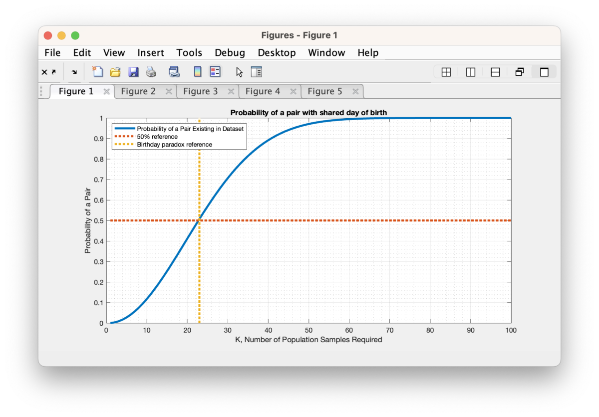
Q: How much of a chance do we actually have of getting an exact (Hamming distance of 0) collision in the full name and full date of birth? Well, there is a similar and well known probability puzzle that asks how many random people do you need to approximately have a 50% chance of 2 of them sharing the same birthday (not including the year of birth). This is known as the “Birthday Problem” in probability theory, and rather surprisingly, the answer is that you only need about 23 people in your population sample to have a 50% probability that 2 of those people will share a day-of-year of birth. To quote the wikipedia article on the matter “… While it may seem surprising that only 23 individuals are required to reach a 50% probability of a shared birthday, this result is made more intuitive by considering that the birthday comparisons will be made between every possible pair of individuals. With 23 individuals, there are 23 × 22/2 = 253 pairs to consider, far more than half the number of days in a year.” The same mathematics of the birthday problem is the basis of the Birthday Attack cryptographic exploit, and it is therefore a well-studied problem in cryptography and cyber security.
Figure 1: The computed probability of at least two people sharing a birthday versus the number of people. A recreation of the classic “Birthday Problem”.
Now, as interesting as the toy birthday problem is as described above, it is over simplified for the problem we are looking at here. Firstly, the problem setup assumes independent and identically distributed random variable (e.g. an “IID” set of variables). While this is not exactly the case, the IID assumption provides for a computable first order estimate, and in the case of the classical birthday problem the estimate has been shown to be fairly accurate under experimental conditions.
Secondly, when we start additionally considering the year of birth, or sharing of first names, middle names and last names, things get much more complicated to compute, but the method is the same. We want to determine the probability of 2 people sharing the same First Name, Middle Name, Last Name, Suffix, Month-of-Birth, Day-of-Birth and Year-of-Birth in the population of unique registrants in the Registered Voter List. This means that in addition to the 365 day-of-birth possibilities, we need to estimate the number of possible years to cover, the number of possible first names, the number of possible middle names, the number of possible last names, the number of possible suffix strings and then include these possibilities into the same formulation as the birthday problem setup.
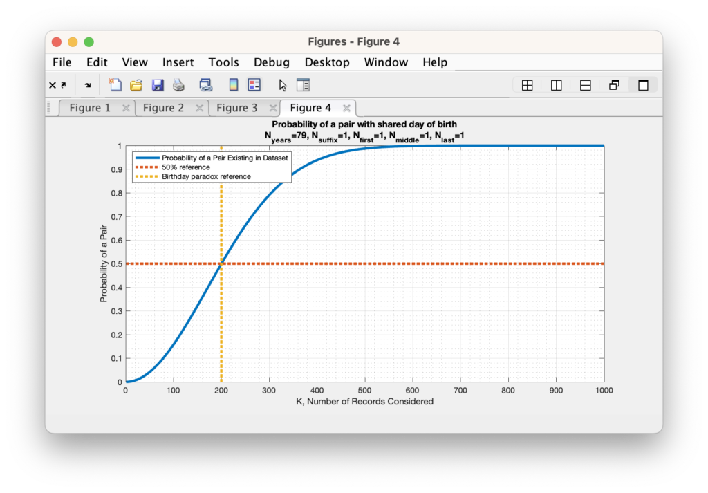
For determining how many years we should cover, I will simply use the average life expectancy of approximately 79 years. We can therefore update our N value of the birthday problem from 365 to 365 * 79 = 28835. When we perform the same analysis as the standard birthday problem with just this new parameter included, we end up needing 200 people in our sample population to have a 50% probability of of 2 people having a match.
Figure 2: The computed probability of at least two people sharing a birthday versus the number of people in the sample population. A recreation of the classic “Birthday Problem”, but we’ve updated the analysis to include the year of birth, and assumed the average life expectancy of 79 years. This moves the 50% crossover point to a population size of 200 from 23 for the standard Birthday Problem setup. [Edit: On 2025-05-13 this plot was corrected to the correct plot. The previous version had repeated the plot of Figure 1.]
A similar analysis can be done with the number of names being considered, etc. For each (assumed independent and uniform) variable we add to the setup, we multiply the number of possible states (N) by the number of unique variable settings.
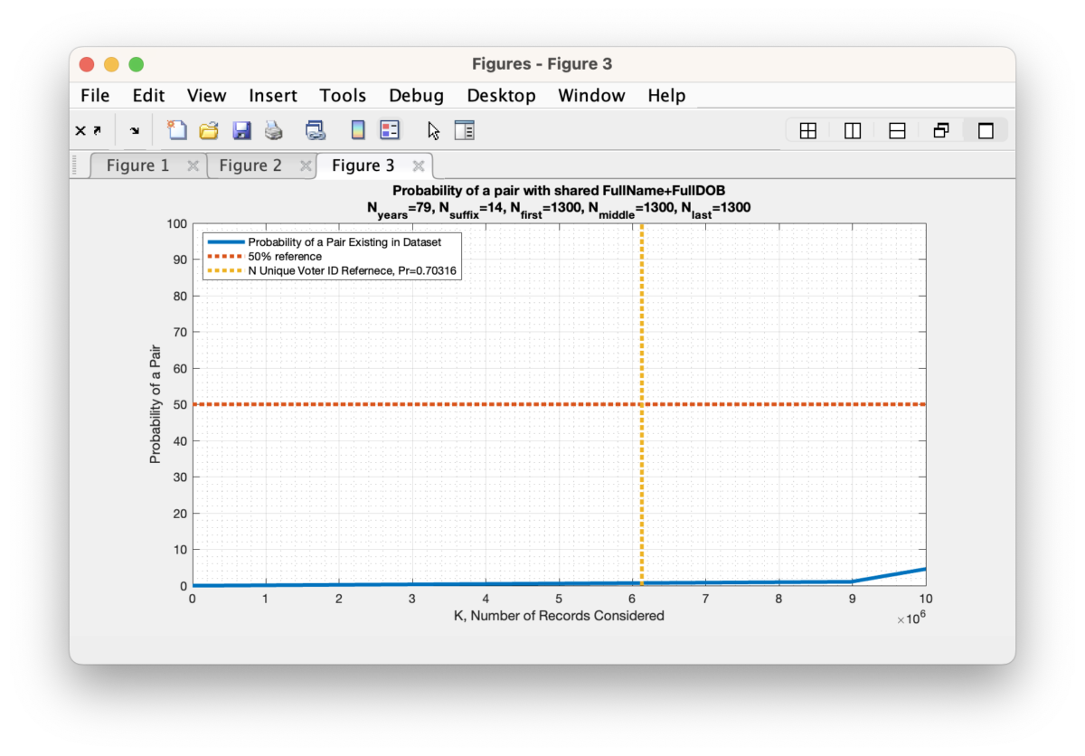
We can estimate the universe of possible names using the frequentist method from the RVL data itself: We know that we have 6,127,859 unique voter ID’s in the RVL, and there are 14 unique SUFFIX entries, 291,368 unique FIRST names, 405,591 unique MIDDLE names, and 465,185 unique LAST names. So multiplying out 365 x 79 x 14 x 291368 x 405591 x 465185 = 2.22 x 10^22 potential states to consider.
Now unfortunately, as we start dealing with bigger and bigger N values the ability of computers to maintain the necessary precision to carry out the mathematics for direct computation becomes harder and harder, eventually resulting in Infinite or divide-by-zero answers as the probabilities get smaller and smaller. So lets begin by first determining if we can find the 50% crossover point for the unique voter ID population size. We find that we only need 410 unique First, Middle, and Last names (each) to break the 50% probability limit.
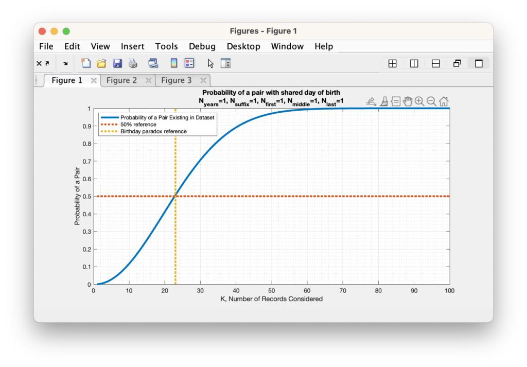
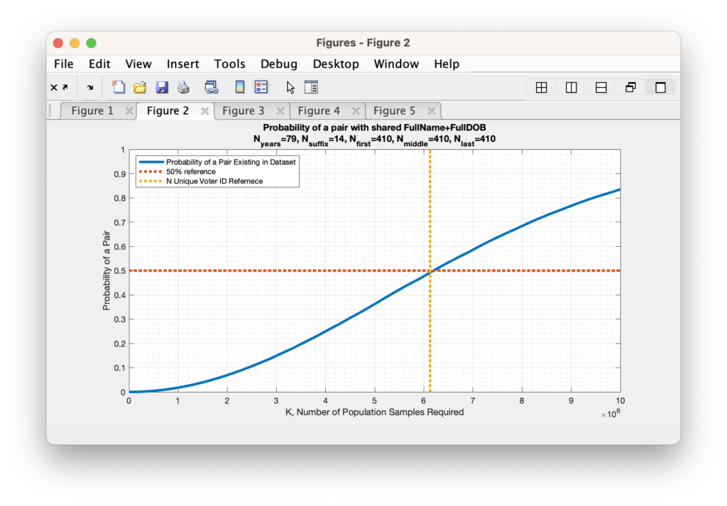
Figure 3: The computed probability of at least two people sharing a first name, middle name, last name, suffix, month-of-birth, day-of-birth, year-of-birth versus the number of people in the sample population. This assumes the Nyears = 79, Nsuffix = 14, Nfirst = 410, Nmiddle = 410, Nlast = 410.
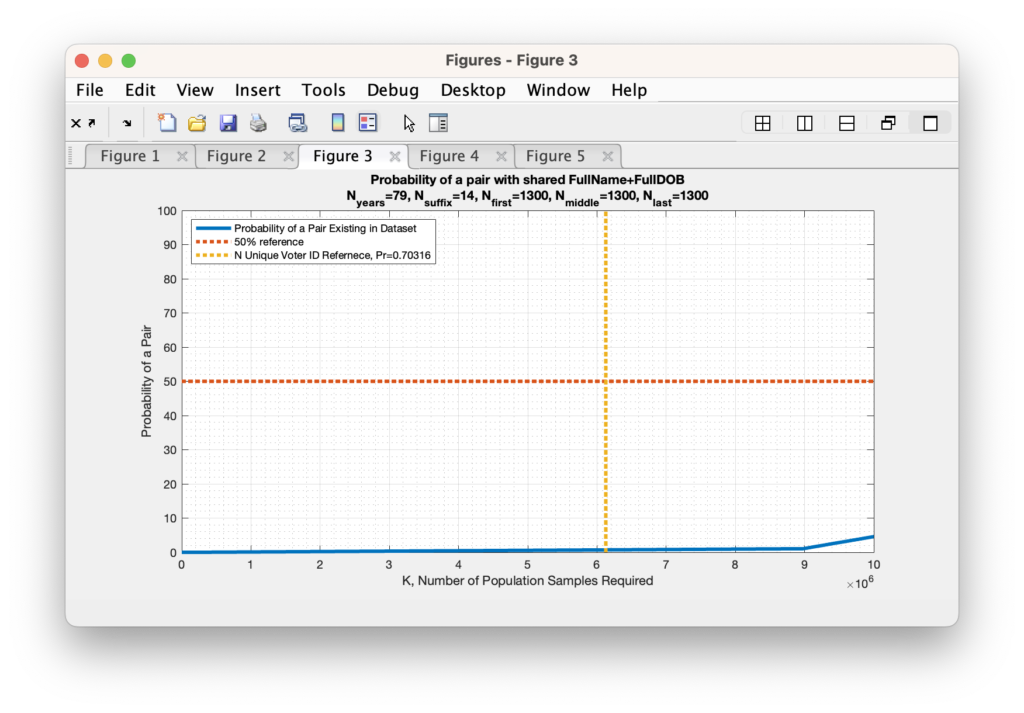
As we increase the number of unique (first, middle, last) names under consideration, we find that we very quickly reduce the probability to near zero (again … this is assuming an IID set of variables … more on that later). In fact we only need to assume that there are 1300 unique first names, middle names and last names before the probability drops to under 1%. This is two full orders of magnitude below the actual number of unique first names, middle names and last names (each) that we find by simple examination of the RVL file, so the actual probability of a collision under these conditions should be much, much, much lower. While not exactly zero, it is computationally indistinguishable from zero given machine precision. Note (again) that this formulation is still simplified in that it assumes a uniform distribution within the N possible states, but it still serves to give a first order approximation and sanity check.
Figure 4: The computed probability of at least two people sharing a first name, middle name, last name, suffix, month-of-birth, day-of-birth, year-of-birth versus the number of people in the sample population. This assumes the Nyears = 79, Nsuffix = 14, Nfirst = 1300, Nmiddle = 1300, Nlast = 1300.
As we start approaching the limit of computational precision we have to resort to approximation methods for computing the very small, but non-zero probability of collision given the actual number of unique first, middle and last names observed in the RVL dataset. We can use the Taylor series expansion for small powers in order to do this, and our equation for computing the probability becomes: Pb = 1 – exp(-k*(k-1) / (2 *N)).
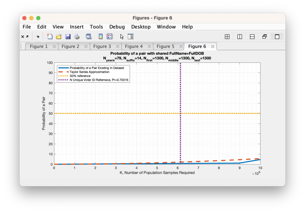
Replicating our earlier example in Figure 4 above with Nfirst == Nmiddle == Nlast == 1300 to show the comparison of the Taylor expansion to the explicit computation produces the graphic in Figure 5 below. We see that the small value approximation is close, but slightly over-estimates the directly computed probability for IID variables.
Figure 5: The computed probability of at least two people sharing a first name, middle name, last name, suffix, month-of-birth, day-of-birth, year-of-birth versus the number of people in the sample population. This assumes the Nyears = 79, Nsuffix = 14, Nfirst = 1300, Nmiddle = 1300, Nlast = 1300.
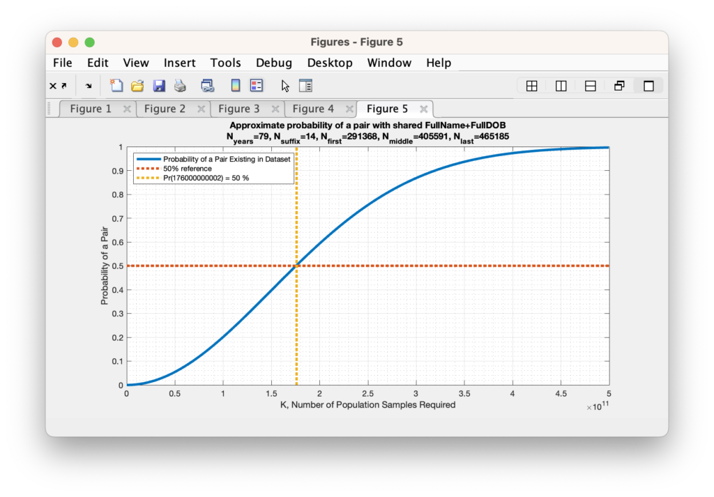
When we perform this Taylor series approximation and look to find the number of records required in order to obtain a 50% probability that any 2 records would match given our updated universe of possible matches, we end up with requiring K = 176,000,000,000, or 176 Billion records. When we again try to evaluate the Taylor series for the explicit number of unique Voter ID’s present in the RVL file, which is just over 6M, we again obtain a number that is computationally indistinguishable from 0. (To be absolutely meticulous … its a bigger number that is indistinguishable from 0 than we previously computed, but it is still indistinguishable from zero.)
Figure 5: The computed probability of at least two people sharing a first name, middle name, last name, suffix, month-of-birth, day-of-birth, year-of-birth versus the number of people in the sample population. This assumes the Nyears = 79, Nsuffix = 14, Nfirst = 291368, Nmiddle = 405591, Nlast = 465185, and the computed 50% crossover point occurs at approximately 176 Billion samples required.
Another Implementation note: In order to explicitly code the above direct computations we also need to do some clever tricks with logarithms in order to avoid numerical overflow / underflow issues as much as possible. The formula for computing the permutations, which is N! / (N-K)! = N x (N-1) x … x (N-K+1) can have numerical issues when N becomes large. However if we take the base-10 logarithm of the equation, we can use the product and quotient rules of logarithms to compute the result and avoid numerical overflow: log10( N! / (N-K)! ) = log10(N!) – log((N-K)!) = log10(N) + log10(N-1) + … + … log10(N-K+1), which is a much more stable computation.
We can perform a similar trick in order to compute the denominator of N^k by using the power property of logarithms such that log10( N^k ) = k x log10(N).
You must of course remember to reverse the logarithm once you’ve computed the log-sums. So the final computation of Pb becomes the following:
Vnr = log10(N) + log10(N-1) + … + … log10(N-K+1), where N is the number of possible states N = 365 x Nyears x Nfirst x Nmiddle x Nlast x Nsuffix.
Vt = k x log10(N)
Pa_log10 = Vnr – Vt = log10(Pa) = log10(Vnr/Vt)
Pb = 1 – 10^(Pa)
Updating from uniform distributions to non-uniform distributions
So what happens when we take into account the fact that names and birthdays are not uniformly distributed? (e.g. the last name of “Smith” is more frequent than “Sandeval”) This fact increases the probability of a collision occurring in the dataset. This increase also makes intuitive sense as we can anecdotally observe that coincident names and birthdates, while still rare … do actually happen in real life with common names.
However, in the non-uniform case we don’t have as nearly of a nice closed set of formulas for computing the probability. What we can do instead to estimate the probability is perform a number of Monte Carlo simulations of selecting K values from the weighted possibilities, and determine how many collisions occurred in each simulation trial. By setting K equal to the number of unique Voter ID values in the RVL dataset, we can directly answer the question via simulation of “how many collisions of First+Middle+Last+Suffix+DOB should we expect when looking at the VA Registered Voter List file“?
We can determine the weightings for each variable easily enough from the distributions of unique values in the data itself.
The below MATLAB weightedCollisionSim(…) function is a program that can be used to perform this analysis. It assumes that the RVL table object is a global variable to setup the trials, and uses the MATLAB built-in randsample(…) function to perform each draw.
After 100 simulation runs, the results are that for the K=6,127,859 unique voter ID’s in the RVL, we should expect to have an average of about 11 collisions at Hamming distance of 0, with a standard deviation of roughly 3.
I will note that as a validation and verification step, the MATLAB simulation code below, when used with uniform sampling, produces similar results to what we analytically derived above.
function [p,m,s] = weightedCollisionSim(k,ntrials,varargin)
% To compute the probability the ntrials must be >> 1:
% [p,m,s] = weightedCollisionSim(k,ntrials,values1,weights1,...,values2,weights2)
% [p,m,s] = weightedCollisionSim(k,ntrials,Nvalues1,weights1,...,Nvalues2,weights2)
%
% OUTPUTS:
% p = Probability of a collision
% m = mean number of collisions
% s = standard deviation of collisions

if nargin == 0
    global rvl; % Assume the RVL is an available global var

    ntrials = 100; % Number of trials

    % Population size set as num of unique voter IDs in RVL
    npop = numel(unique(rvl.IDENTIFICATION_NUMBER));

    % Convert the DOB strings to datetime objects
    dob = datetime(rvl.DOB);

    % How many unique days of the year are there?
    [ud,uda,udb] = unique(day(dob,'dayofyear'));
    % How often do they occur?
    nud = accumarray(udb,1,[numel(ud),1]);
    Ndays = numel(ud);

    % How many unique years of birth are there?
    [uy,uya,uyb] = unique(year(dob));
    % How often do they occur?
    nuy = accumarray(uyb,1,[numel(uy),1]);
    Nyears = numel(uy);

    % How many unique suffix strings are there?
    [us,usa,usb] = unique(rvl.SUFFIX);
    % How often do they occur?
    nus = accumarray(usb,1,[numel(us),1]);
    Nsuffix = numel(us);

    % How many unique first names are there?
    [uf,ufa,ufb] = unique(rvl.FIRST_NAME);
    % How often do they occur?
    nuf = accumarray(ufb,1,[numel(uf),1]);
    Nfirst = numel(uf);

    % How many unique middle names are there?
    [um,uma,umb] = unique(rvl.MIDDLE_NAME);
    % How often do they occur?
    num = accumarray(umb,1,[numel(um),1])
    Nmiddle = numel(um);

    % How many unique last names are there?
    [ul,ula,ulb] = unique(rvl.LAST_NAME);
    % How often do they occur?
    nul = accumarray(ulb,1,[numel(ul),1]);
    Nlast = numel(ul);

    % Initializing the weighting vectors
    w0 = nus;
    w1 = nud;
    w2 = nuy;
    w3 = nuf;
    w4 = num;
    w5 = nul;

    % Recursively compute results and return
    [p,m,s] = weightedCollisionSim(npop,ntrials,1:Nsuffix,w0,1:Ndays,w1,1:Nyears,w2,...
        1:Nfirst,w3,1:Nmiddle,w4,1:Nlast,w5);
    return
end

if nargin < 2 || isempty(ntrials)
    ntrials = 1;
end

nc = zeros(ntrials,1);
for j = 1:ntrials
    fprintf('Trial %d\n',j);
    y = zeros(k,numel(varargin)/2);
    m = 1;
    for i = 1:2:numel(varargin)
        w = varargin{i+1};
        v = varargin{i};
        if ~isempty(w) && isvector(w)
            % Non-uniform weightings
            y(:,m) = randsample(v,k,true,w);
        else
            % Uniform sampling
            y(:,m) = randsample(v,k,true);
        end
        m = m+1;
    end
    [u,~,ib] = unique(y,'rows');
    nu = accumarray(ib,1,[size(u,1),1]);
    nc(j) = sum(nu > 1);
end
p = mean(nc>0);
m = mean(nc);
s = std(nc);
Per the recent James O’Keefe video documenting incredulous amounts of contributions by individuals to political committees, I took a few minutes to download the public FEC data in bulk format and collated all of the individuals that had more than 100 donations to each of the following organizations: DNC, DCCC, DSCC, RNC, NRSC, NRCC, WinRed, ActBlue in the 2021-2022 Election period.
I made sure to account for and remove those records of contributions that had been (legally) returned due to over-contribution, or earmarked for campaign committee legal or facility funds, etc which are exempt from campaign finance limits.
I hope it helps James. I’m not going to try and do any sort of analysis on this data, as I’ve got plenty to do regarding the IT of our elections, but I wanted to help where I could. Any questions, or if you would like the raw transaction data, please feel free to contact me, or if you have a particular committee ID that you would like the information for, just let me know. I am happy to help.
Using the 2022-11-23 Registered Voter List (RVL) and the 2023-01-26 Voter History List (VHL) purchased from the VA Department of Elections (ELECT) I wrote up an analysis script to check for potentially duplicated registrant records in the RVL and cross reference duplicate pairings with the VHL to identify potential duplicate votes. This was my initial attempt at quantifying the number of potentially duplicate records in the RVL, and I have since updated the code to use a more rigorous Levenshtein distance metric, as well as making improvements to the parsing routines, bugfixes, etc. The details of the Hamming distance work are summarized below, and left up here for reference. For the latest and up to date information, please see the newer article posted here.
Errata note: One of the code bugs I discovered was that some of the entries did not actually get checked as they were accidentally skipped, so the numbers below are lower than the numbers presented in the newer work.
Please note that I will not publish voter Personally Identifiable Information (PII) on this blog. I have substituted fictitious PII information for all examples given below, and cryptographically hashed all voter information in the downloadable results file. I will make available the detailed information to those that have the authorization to receive and process voter data upon request (contact us).
Summary of Results:
We should mathematically expect approximately 11 exact string collisions in the full RVL dataset when comparing (First Name + Middle Name + Last Name + Suffix + Full DOB), but instead we see 1982 such collisions, which is over an order of magnitude increase from the expected value. While its possible that some of these collisions are false positives, there are quite a number of them that are deserving of further scrutiny.
Method:
For every entry in the latest RVL, I performed a string distance comparison, based on Hamming distance, between every possible pair of strings of (FIRST NAME + MIDDLE NAME + LAST NAME + SUFFIX + FULL DOB). So for the ~6M different RVL entries, we need to compute ~3.6 x 10^13 different string comparisons. A hamming distance of 0 indicates the strings being compared are identical, a hamming distance of 1 indicates that there is a single character different between the two strings, a hamming distance of 2 indicates 2 characters are different, etc. This obviously is a very computationally intensive process and it took over two days to complete the processing, once I got the bugs worked out. (I’ve been quietly working on this one for a while now … )
Note that the Hamming distance only compares each respective position in a string and does not account for adding or removing a character completely from a string. A metric that does include addition and subtraction is the Levenshtein Edit Distance, which is much more computationally expensive (but more rigorous) metric. The Hamming distance is related to the Levenshtein distance in that it is mathematically the upper bound on the Levenshtein distance for arbitrary strings. I haven’t yet finished making an optimized GPU accelerated version of the Levenshtein edit distance metric, but it is in the works and I will redo this analysis with the new metric once that is completed.
I aggregated all of the Hamming distance pairings that were less than or equal to 3 characters different in order to identify potential (key word) duplicated registrants, and additionally for each pairing looked at the voter history information for each registrant in the pair to determine if there was a potential (again … key word) for multiple ballots to be cast by the same person in any given election. As we allow for more characters to be different, we potentially are including many more likely false positive matches, even if we are catching more true positives.
For example: At a Hamming distance of 4 the strings of “Dave Joseph Smith M 10/01/1981” and “Tony Joseph Smith M 10/01/1981” at the same address would produce a potential match, but so would “Davey Joseph Smith M 10/01/1981” and “David Josiph Smith M 10/02/1981”. The first pair is more likely to be a false positive due to twins, while the second is more likely to be due to typo’s, mistakes, or use of nicknames and might warrant further investigation. A much stronger potential match would be something like “David Josiph Smith M 10/01/1981” and “David Joseph Smith M 10/01/1981”, with a Hamming distance of 1 at the same address. In an attempt to limit false positives, I have clamped the Hamming distance checks to <= 3 in this analysis.
One of the drawbacks of using Hamming distance over a more complete metric such as Levenshtein, is that the Hamming distance would give a very high score, and would therefore filter out of our results, an example pairing such as: “David Joseph Smith M 10/01/1981” and “Dave Joseph Smith M 10/01/1981”. The change from “id” to “e” adds/subtracts a character making the rest of the characters in the remainder of the string shift position and also not match. A Levenshtein metric would correctly return a small distance of 2, whereas the hamming distance returns 27. (As mentioned earlier, I am working on a Levenshtein implementation, but it is not yet complete.)
Note that with the official records obtained from ELECT, and in accordance with the laws of VA, I do not have access to the social security number or drivers license numbers for each registration record, which would help in identifying and discriminating potential duplicate errors vs things like twins, etc. I only have the first name, middle name, last name, suffix, month of birth, day of birth, year of birth, gender, and address information that I can work with. I can therefore only take things so far before someone else (with investigative authority and ability to access those other fields) would need to step in and confirm and validate these findings.
Results:
The summary totals are as follows, with detailed examples.
Hamming Distance
0
1
2
3
Number of Potential Duplicate Registrant Pairs
1982
3276
21864
120642
Number of Potential Duplicate Ballots
110
3248
31210
175872
According to my derivations and simulations that are described in detail at the end of this article, we should only expect to see an average of 11 (+/- 3) potential duplicate pairs (a.k.a. “collisions”) at a Hamming distance of 0. This is over two orders of magnitude different than what we observe in the compiled results table above. Such a discrepancy deserves further investigation and verification.
Examples of Types of Issues Observed:
NOTE THE BELOW INFORMATION HAS HAD THE VOTER PERSONALLY IDENTIFIABLE INFORMATION (“PII”) FICTIONALIZED. WHILE THESE ARE BASED ON REAL DATA TO ILLUSTRATE THE DIFFERENT TYPES OF OBSERVATIONS, THEY DO NOT REPRESENT REAL VOTER INFORMATION.
Example #1: The following set of records has the exact match (Hamming Distance = 0) of full name and full birthdate (including year), but different address and different voter ID numbers AND there was a vote cast from each of those unique voter ID’s in the 2020 General Election. While it’s remotely possible that two individuals share the exact same name, month, day and year of birth … it is probabilistically unlikely (see section below on mathematical derivation of probabilities if interested), and should warrant further scrutiny.
Voter Record A:
AMY BETH McVOTER 12/05/1970 F 12345 CITIZEN CT
Voter Record B:
AMY BETH McVOTER 12/05/1970 F 5678 McPUBLIC DR
Example #2: This set of records has a single character different (Hamming distance of 1) in their first name, but middle name, last name, birthdate and address are identical AND both records are associated with votes that were cast in the 2020, 2021, and 2022 November General Elections. While it is possible that this is a pair of 23 year old twins (with same middle names) that live together, it at least bears looking into.
Voter Record A:
TAYLOR DAVID VOTER 02/16/2000 M 6543 OVERLOOK AVE NW
Voter Record B:
DAYLOR DAVID VOTER 02/16/2000 M 6543 OVERLOOK AVE NW
Example #3: This set of records has two characters different (Hamming distance of 2) in their birthdate, but name and address are identical AND the birth years are too close together for a child/parent relationship, AND both records are associated with votes that were cast in the 2020 and 2022 November General Elections.
Voter Record A:
REGINA DESEREE MACGUFFIN 02/05/1973 F 123 POPE AVE
Voter Record B:
REGINA DESEREE MACGUFFIN 03/07/1973 F 123 POPE AVE
Example #4: This set of records has again a single character different (Hamming distance of 1) in the first name (but not the first letter this time) and the last name, birthdate and address are identical. There were also multiple votes cast in the 2019 and 2022 November General from these registrants.
Voter Record A:
EDGARD JOHNSON 10/19/1981 M 5498 PAGELAND BLVD
Voter Record B:
EDUARD JOHNSON 10/19/1981 M 5498 PAGELAND BLVD
Example #5: This set of records has two characters different (Hamming distance of 2) in the first and middle names and the last name, birthdate, gender and address are identical. There were also multiple votes cast in the 2021 and 2022 November General from these registrants. Again it is possible that these records represent a set of twins given the information that ELECT provides.
Voter Record A:
ALANA JAVETTE THOMPSON 01/01/2003 F 123 CHARITY LN
Voter Record B:
ALAYA YAVETTE THOMPSON 01/01/2003 F 123 CHARITY LN
Example #6: The following set of records has the exact match (Hamming Distance = 0) of full name and full birthdate (including year), and same address but different voter ID numbers. There was no duplicated votes in the same election detected between the two ID numbers.
Voter Record A:
JAMES TIBERIUS KIRK 03/22/2223 M 1701 Enterprise Bridge
Voter Record B:
JAMES TIBERIUS KIRK 03/22/2223 M 1701 Enterprise Bridge
Example #7: The following set of records has the exact match (Hamming Distance = 0) of full name and full birthdate (including year), same address but different gender and voter ID numbers. There was no duplicated votes in the same election detected between the two ID numbers.
Voter Record A:
MAXWELL QUAID CLINGER 11/03/2004 M 4077 MASH DR
Voter Record B:
MAXWELL QUAID CLINGER 11/03/2004 U 4077 MASH DR
Results Dataset:
A full version of the aggregated excel data is provided below, however all voter information (ID, first name, middle name, last name, dob, gender, address) have been removed and replaced by a one-way hash number, with randomized salt, based on the voter ID. The full file with specific voter information can be provided to parties authorized by ELECT to recieve and process voter information, Election Officials, or Law Enforcement upon request.
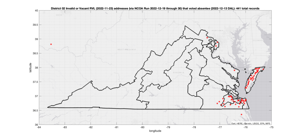
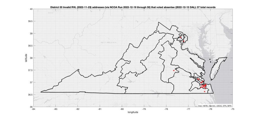
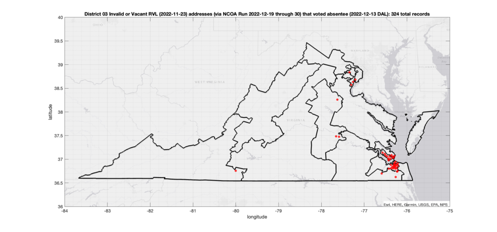
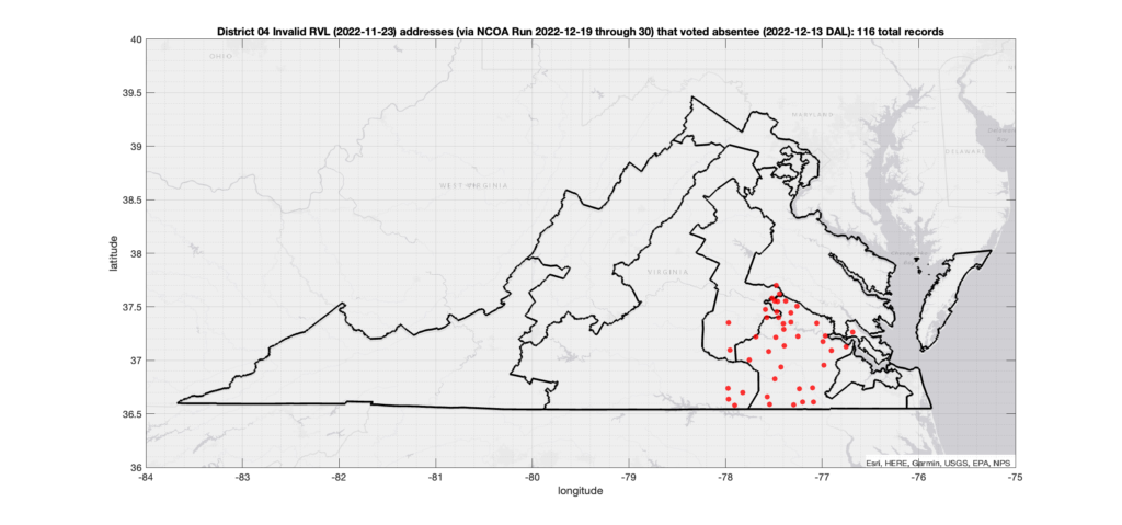
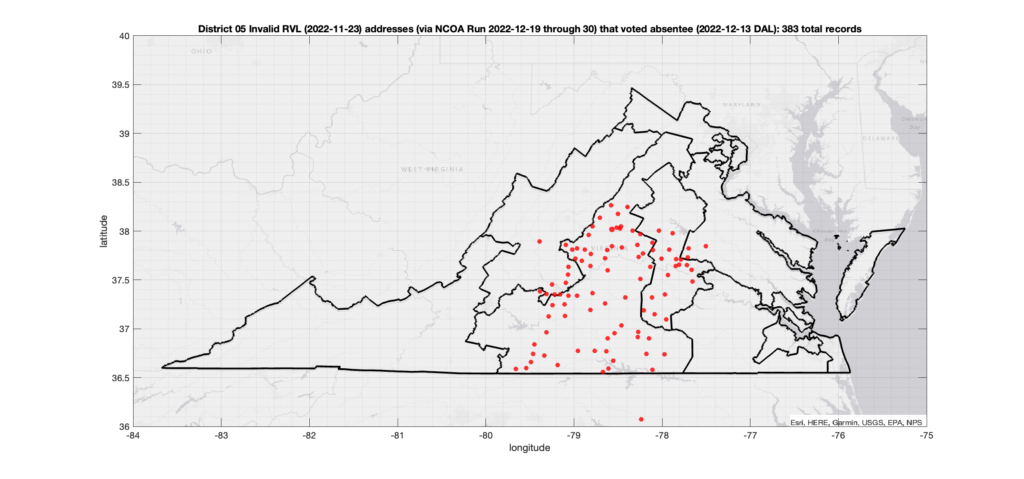
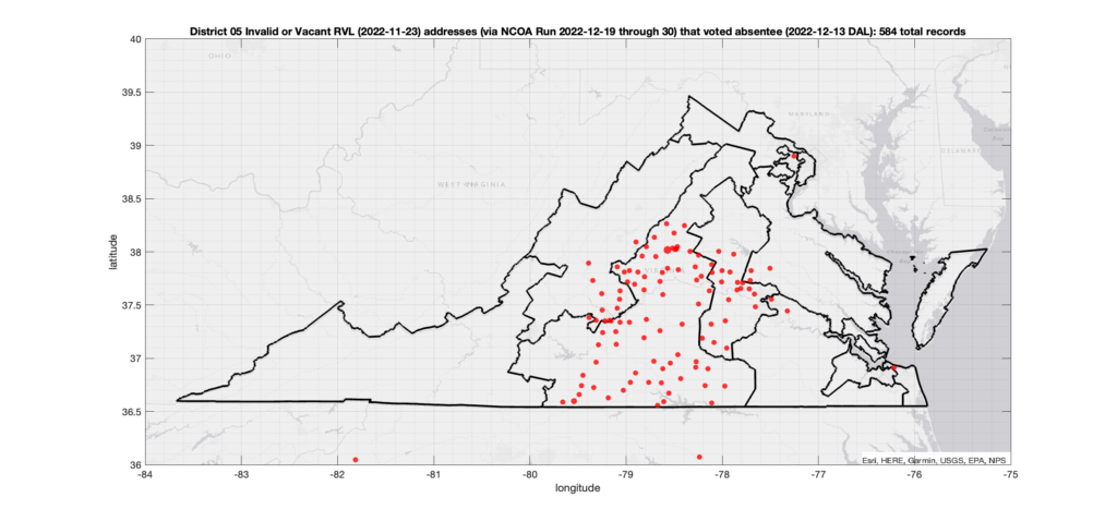
In a previous post I documented the results from an United States Postal Service (USPS) National Change of Address (NCOA) database check with the 2022 Virginia Registered Voter List (RVL) primary address records joined with the Daily Absentee List (DAL) reports of absentee ballots cast. There was a significant public reaction to the fact that over 15K RVL primary addresses associated with voters who cast ballots in the VA 2022 general election were not recognized by the USPS database as valid addresses (among other issues). I reported the data as I found it, but a common commentary was that my analysis did not account for rural voters who do not have a traditional street address, or that do not have mail receptacles and use PO boxes as their primary delivery mechanism.
The requirements for voter registration and primary address are specified by the VA Constitution, Federal and VA law, and require the following:
The VA constitution (Section II-1 and II-2) and the National Voter Registration Act (NVRA) requires that registered voter primary addresses be an actual physical (and deliverable) street address. The de-facto arbiter of what defines a recognizable and/or deliverable address is the USPS, therefore a street address that is not recognized or is undeliverable according to USPS is not compliant. We should be making every effort to ensure that the primary address associated with each voter is able to be correctly recognized and translated into a deliverable address by the USPS. This may require adjusting VA’s data normalization policies such that input street addresses are correctly mapped to USPS addresses, or a legislative action in order to correct.
There is also the legal restriction that registered VA voters are not allowed to use PO Boxes as their primary registered voter address. There is an exception that “protected” voters are allowed to provide a PO box address to be displayed in public records, but their actual address on file must still be a physical address.
The 2022 VA GREB, section 6..2.3 states that in special cases, a rural voter may supply the name of the highway and enough detail in the comments section of the voter application that the registrar may ascertain where the physical address is. This seems (IMO, but I’m not a lawyer) in contradiction to the language in the VA constitution and in the NVRA that make the implicit requirement of deliverable addresses. Also, if the address as entered is not recognized by the USPS NCOA system, then it will constantly be generating validation errors every time it is checked against the NCOA database, which VA is currently required to do at least annually. Again, this may require adjusting VA’s data normalization policies such that input street addresses are correctly mapped to USPS addresses, or a legislative action in order to correct.
Additionally the USPS is supposed to recognize “Post Box Street Address” (PBSA) locations such that when someone addresses an envelope or package to the street address of a residence that is served only by delivery to a PO box, the USPS should automatically recognize this and adjust accordingly. Per the NCOA documentation, the USPS NCOA database checks are supposed to be doing this detection and translation already.
And again, to be clear, my point is not to accuse anyone of malicious intent or wrongdoing … I am simply trying to point out that the way we are using and managing our data is discrepant with what the requirements actually are. We either need to change the data and our practices to conform to the legal requirements, or change the law to fit how we are actually (and practically) using the data.
That being said, and in order to show that there are still significant data issues even after adjusting for rural routes, etc., I’ve re-run my NCOA analysis to account for records with invalid primary addresses but that had valid mailing addresses, even if those mailing addresses are PO Boxes. Any RVL record with a primary address that was marked invalid by an NCOA check, but had a different mailing address AND that mailing address was returned from a second NCOA check as NOT-invalid (even if it was a PO Box), was replaced with the mailing address listing and NCOA results. While the requirement is still that primary addresses are supposed to be valid, this re-processing and allowing for primary OR mailing addresses to be used is more in line with the way VA has actually implemented its voter registrations across the state … even though that implementation seems to be at odds with the requirements.
The rest of the analysis is performed the same as before, and is presented in the same format for consistency. I have updated the dates and numerical results as appropriate, but have otherwise kept the format and much of the language and layout the same as the previous analysis.
BLUF (Bottom Line Up Front):
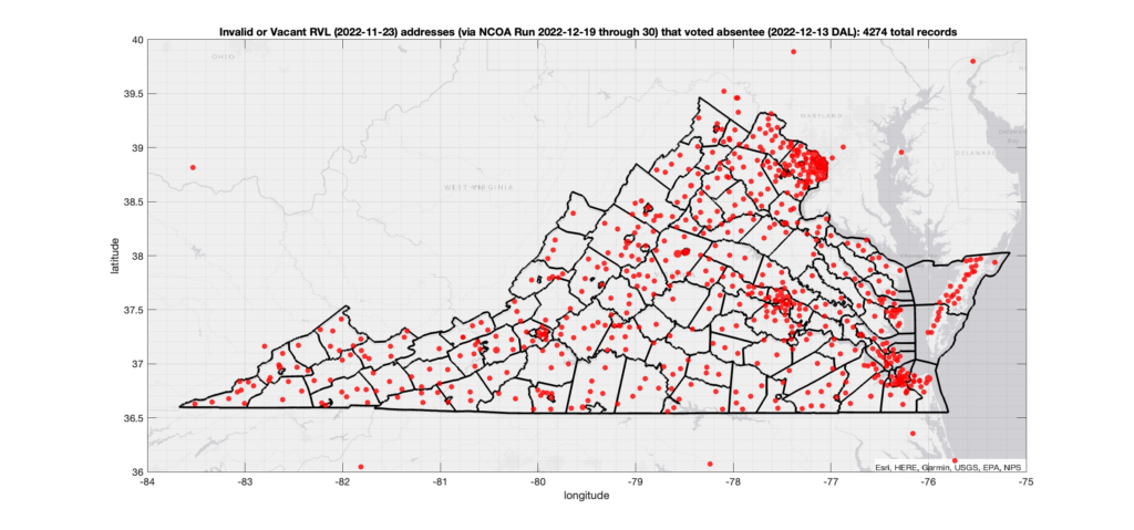
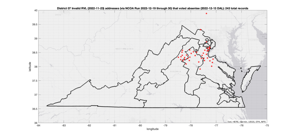
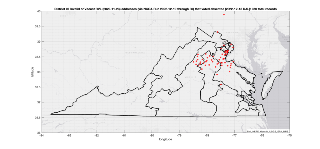
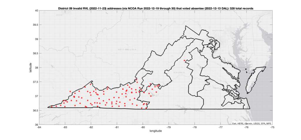
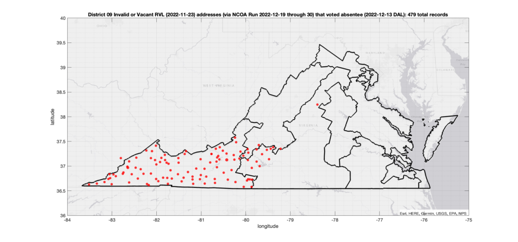
There were 2,164 ballots cast during early voting in the VA 2022 General Election where the voters’ (primary or mailing) registered address on record were flagged as “Invalid” by a National Change of Address (NCOA) database check. If we include addresses that were identified as 90-day Vacant the total rises to 4,274. (The previous analysis that used only the primary addresses returned 15,419 invalid records with associated ballots, and went up to 17,244 when including addresses flagged as vacant.)
A certified commercial provider of NCOA data verification was used to facilitate this analysis on raw data obtained from the VA Dept of Elections (“ELECT”). It is not technically possible to obtain a truly time-synchronized complete set of data for any election due to the way elections are run in VA, but we made every effort to obtain the data from the state as close in time as was possible. The NCOA database is maintained and curated by the United States Postal Service (USPS).
For those wishing to review specific entries, or to help validate these issues, and who are part of an organization that is able to receive and handle election information according to VA law and the VA Dept of Elections requirements, you may contact us to request the raw data breakdowns. We will need to validate your organization or employment and will make data available as legally allowed.
Commentary and Discussion:
I would like to be very clear: We are simply presenting the data as compiled to facilitate public discourse. We have strived to only utilize data directly obtained from authoritative sources (ELECT, the USPS via TrueNCOA provider).
The designation of “Invalid” addresses is according to the definition by the USPS and TrueNCOA, i.e. the TrueNCOA check has reported the addresses as listed in the RVL have no match in the USPS database. Invalid addresses do not include things like valid P.O. Boxes or valid rural addresses that are automatically recognized and translated by USPS to Post Box Street Address (PBSA) records.
The VA Constitution (Section II-1 and II-2) specify the requirements for voter eligibility to include that voters are required to supply a primary address for their registration record, regardless of their method of voting. VA is required by law to consistently maintain and validate these records. Based on the below analysis, the data shows that there is a small but statistically significant number of “Invalid” addresses associated for voters who cast ballots in the Nov 2022 election.
Continuing EPEC’s mission to promote voter participation, analyze election technology, and educate the public about best practices in managing election technology systems; we are providing the below analysis in order to educate and inform the public, legislators and elections officials about the existence of these discrepancies.
Details:
After receiving the results of a National Change of Address (NCOA) database check on the registration (not the temporary) addresses in the latest VA Registered Voter List (RVL). I’ve gone through and collated the flagged addresses and reconciled them with the entries in the Daily Absentee List (DAL) file records provided by the VA Dept. of Elections (“ELECT”).
The DAL file (dated 2022-12-13) provides a records of all of the voters that cast absentee (either Early In-Person or Mail-In) ballots in the election, and the RVL (dated 2022-11-23) gives all of the registered voter addresses and other pertinent information. Both datasets come directly from the VA Dept. of Elections and must be purchased. Total cost was ~$7000. The two datasets can be tied together using the voter Identification Number that is assigned to each (supposedly) unique voter by the state. Entries in the RVL should be unique to each registered voter (although there are a small number of duplicate voter IDs that I have seen … but thats for another post), whereas the DAL file can have multiple entries attributed to a single voter recording the various stages of ballot processing.
The NCOA check was performed on all addresses in the RVL file in order to detect recent moves, invalid addresses, vacant addresses, P.O. Boxes, commercial addresses, etc. The NCOA check takes multiple days to run using a commercial service provider and was executed between 2022-12-19 through 2022-12-30.
*** As noted above, in this run I substituted those primary addresses that evaluated to “invalid” with their corresponding “mailing” address records that had been recognized as “valid”, if possible. ***
Results:
Raw TrueNCOA Processing result stats on the full RVA dataset:
NCOA Processing of VA RVL Records
Full RVL 11-23 Primary Addresses (12/30/2022)
%
Unique RVL Mailing Addresses (12/30/2022)
%
Records Processed
6,127,856
216,896
18 – Month NCOA Moves
282,669
4.61%
8,247
3.80%
48 – Month NCOA Moves
163,931
2.68%
8,099
3.73%
Moves with no Forwarding Address
20,913
0.34%
1,415
0.65%
Total NCOA Moves
467,513
7.63%
17,761
8.19%
Vacant Flag
29,315
0.48%
22,763
10.49%
DPV Updated/Address Corrected Records
601,539
9.82%
18,555
8.55%
DPV Deliverable Records
5,835,230
95.22%
165,939
76.51%
DPV Non-Deliverable Records
185,752
3.03%
35,100
16.18%
LACS Updated (Rural Address converted to Street Address)
33,497
0.55%
254
0.12%
Residential Delivery Indicator
5,970,531
97.43%
194,342
89.60%
Addresses matched to the USPS Database
6,020,983
98.26%
201,040
92.69%
Invalid Addresses
107,304
1.75%
15,968
7.36%
Expired Addresses
10,822
0.18%
276
0.13%
Business Move (B)
340
0.01%
61
0.03%
Family Move (F)
116874
1.91%
5,390
2.49%
Individual Move (I)
350299
5.72%
12,310
5.68%
General Delivery Address
159
0.00%
170
0.08%
High Rise Address
764922
12.48%
7,097
3.27%
PO Box Address
28040
0.46%
158,359
73.01%
Rural Route Address
81
0.00%
269
0.12%
Single Family Address
5243321
85.57%
33,582
15.48%
Unknown
51903
0.85%
15,537
7.16%
Reporting as presented from the TrueNCOA data service. The TrueNCOA data dictionary is presented here.
Combining NCOA results of RVL Addresses with the DAL data:
Vacant Addresses:
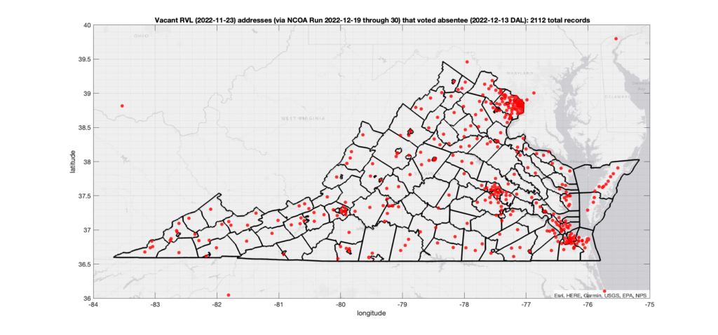
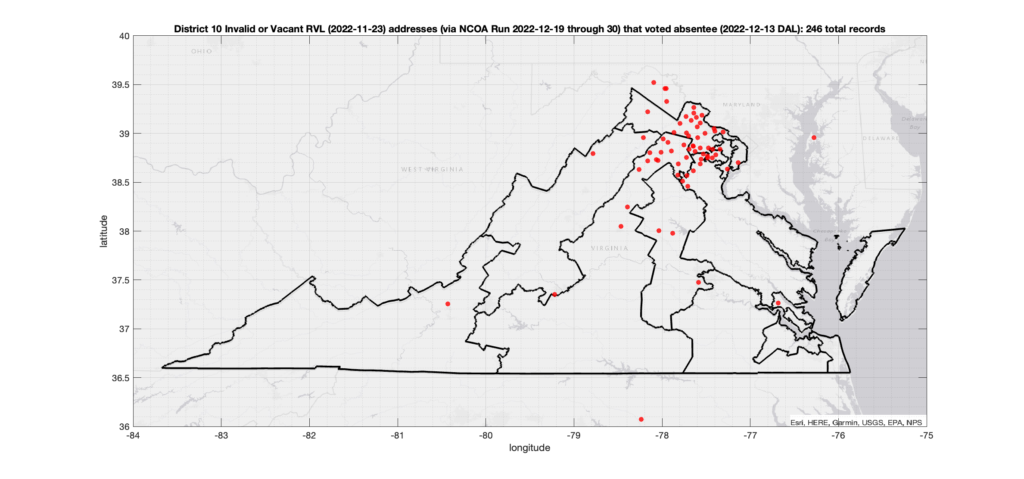
There were 2,112 records across the state with addresses that have been flagged as (90-day) “Vacant” by the NCOA check and also had an Early In-Person, Mail-In, FWAB or Provisional ballot cast in the VA 2022 General Election according to the DAL file. Of those records, 1,542 were Early In-Person and 547 were Mail-In. The geographic distribution of the addresses (based on the ZIP+4), as reported by the NCOA service, is shown below, with the size of the marker proportional to the total number of counts at that ZIP+4 location. (Note this is actually an increase over the previous results that were not adjusted for potential mailing address matches.)
P.O. Boxes (Non-protected):
There were 13,492 records across the state with addresses that have been flagged as P.O. Box Addresses by the NCOA check and also had an Early In-Person, Mail-In, FWAB or Provisional ballot cast in the VA 2022 General Election AND were NOT listed as protected entries according to the DAL file. (VA allows for voters who have a legal protective order to list a P.O. Box as their address of record on public documents) Of those records, 11,426 were Early In-Person and 2020 were Mail-In. The geographic distribution of the addresses (based on the ZIP+4), as reported by the NCOA service, is shown below, with the size of the marker proportional to the total number of counts at that ZIP+4 location.
Note, this is actually an increase over the previous results that were not adjusted for potential mailing address matches. This is not unexpected, as there are a number of PO box mailing addresses that have been substituted in for invalid primary street addresses. PO Boxes are not supposed to be allowed as registered voting addresses. (You should talk to your legislators about this discrepancy, because this catch-22 will likely need to be changed by legislative action!)
Invalid Addresses:
There were 2,164 records across the state with addresses that have been flagged as “Invalid” Addresses by the NCOA check and also had an Early In-Person, Mail-In, FWAB or Provisional ballot cast in the VA 2022 General Election. Of those records, 1,535 were Early In-Person and 598 were Mail-In. The geographic distribution of the addresses (based on the ZIP+4), as reported by the NCOA service, is shown below, with the size of the marker proportional to the total number of counts at that ZIP+4 location. Note, this is actually a significant decrease over the previous results that were not adjusted for potential mailing addresses. This is not unexpected, as there were a number of invalid primary address with a valid (even if PO Box) mailing address. (The fact that the primary addresses do not validate with the USPS is it’s own issue, but we are ignoring that for this analysis as noted above.)
Invalid OR Vacant Addresses:
There were 4,274 records across the state with addresses that have been flagged as “Invalid” or “Vacant” Addresses by the NCOA check and also had an Early In-Person, Mail-In, FWAB or Provisional ballot cast in the VA 2022 General Election. Of those records, 3,077 were Early In-Person and 1,143 were Mail-In. The geographic distribution of the addresses (based on the ZIP+4), as reported by the NCOA service, is shown below, with the size of the marker proportional to the total number of counts at that ZIP+4 location.
Record of Moves Out-of-State:
There were 797 records that had records of NCOA moves to valid out-of-state addresses before 2022-08 that also had an Early In-Person, Mail-In, FWAB or Provisional ballot cast in the VA 2022 General Election. Of those records, 346 were Early In-Person and 450 were Mail-In. The geographic distribution of the addresses (based on the ZIP+4), as reported by the NCOA service, is shown below, with the size of the marker proportional to the total number of counts at that ZIP+4 location.
Results By District:
District 01:
Invalid Addresses:
There were 213 records with registered addresses that have been flagged as “Invalid” Addresses by the NCOA check and also had an Early In-Person, Mail-In, FWAB or Provisional ballot cast in the VA 2022 General Election in District 01. Of those records, 170 were Early In-Person and 38 were Mail-In. The geographic distribution of the addresses (based on the ZIP+4), as reported by the NCOA service, is shown below, with the size of the marker proportional to the total number of counts at that ZIP+4 location.
Invalid OR Vacant Addresses:
There were 364 records with registered addresses that have been flagged as “Invalid” or “Vacant” Addresses by the NCOA check and also had an Early In-Person, Mail-In, FWAB or Provisional ballot cast in the VA 2022 General Election in District 01. Of those records, 288 were Early In-Person and 71 were Mail-In. The geographic distribution of the addresses (based on the ZIP+4), as reported by the NCOA service, is shown below, with the size of the marker proportional to the total number of counts at that ZIP+4 location.
District 02:
Invalid Addresses:
There were 183 records with registered addresses that have been flagged as “Invalid” Addresses by the NCOA check and also had an Early In-Person, Mail-In, FWAB or Provisional ballot cast in the VA 2022 General Election in District 02. Of those records, 147 were Early In-Person and 33 were Mail-In. The geographic distribution of the addresses (based on the ZIP+4), as reported by the NCOA service, is shown below, with the size of the marker proportional to the total number of counts at that ZIP+4 location.
Invalid OR Vacant Addresses:
There were 441 records with registered addresses that have been flagged as “Invalid” or “Vacant” Addresses by the NCOA check and also had an Early In-Person, Mail-In, FWAB or Provisional ballot cast in the VA 2022 General Election in District 02. Of those records, 344 were Early In-Person and 90 were Mail-In. The geographic distribution of the addresses (based on the ZIP+4), as reported by the NCOA service, is shown below, with the size of the marker proportional to the total number of counts at that ZIP+4 location.
District 03:
Invalid Addresses:
There were 37 records with registered addresses that have been flagged as “Invalid” Addresses by the NCOA check and also had an Early In-Person, Mail-In, FWAB or Provisional ballot cast in the VA 2022 General Election in District 03. Of those records, 27 were Early In-Person and 10 were Mail-In. The geographic distribution of the addresses (based on the ZIP+4), as reported by the NCOA service, is shown below, with the size of the marker proportional to the total number of counts at that ZIP+4 location.
Invalid OR Vacant Addresses:
There were 324 records with registered addresses that have been flagged as “Invalid” or “Vacant” Addresses by the NCOA check and also had an Early In-Person, Mail-In, FWAB or Provisional ballot cast in the VA 2022 General Election in District 03. Of those records, 223 were Early In-Person and 94 were Mail-In. The geographic distribution of the addresses (based on the ZIP+4), as reported by the NCOA service, is shown below, with the size of the marker proportional to the total number of counts at that ZIP+4 location.
District 04:
Invalid Addresses:
There were 116 records with registered addresses that have been flagged as “Invalid” Addresses by the NCOA check and also had an Early In-Person, Mail-In, FWAB or Provisional ballot cast in the VA 2022 General Election in District 04. Of those records, 104 were Early In-Person and 12 were Mail-In. The geographic distribution of the addresses (based on the ZIP+4), as reported by the NCOA service, is shown below, with the size of the marker proportional to the total number of counts at that ZIP+4 location.
Invalid OR Vacant Addresses:
There were 318 records with registered addresses that have been flagged as “Invalid” or “Vacant” Addresses by the NCOA check and also had an Early In-Person, Mail-In, FWAB or Provisional ballot cast in the VA 2022 General Election in District 04. Of those records, 256 were Early In-Person and 59 were Mail-In. The geographic distribution of the addresses (based on the ZIP+4), as reported by the NCOA service, is shown below, with the size of the marker proportional to the total number of counts at that ZIP+4 location.
District 05:
Invalid Addresses:
There were 383 records with registered addresses that have been flagged as “Invalid” Addresses by the NCOA check and also had an Early In-Person, Mail-In, FWAB or Provisional ballot cast in the VA 2022 General Election in District 05. Of those records, 299 were Early In-Person and 81 were Mail-In. The geographic distribution of the addresses (based on the ZIP+4), as reported by the NCOA service, is shown below, with the size of the marker proportional to the total number of counts at that ZIP+4 location.
Invalid OR Vacant Addresses:
There were 584 records with registered addresses that have been flagged as “Invalid” or “Vacant” Addresses by the NCOA check and also had an Early In-Person, Mail-In, FWAB or Provisional ballot cast in the VA 2022 General Election in District 05. Of those records, 445 were Early In-Person and 134 were Mail-In. The geographic distribution of the addresses (based on the ZIP+4), as reported by the NCOA service, is shown below, with the size of the marker proportional to the total number of counts at that ZIP+4 location.
District 06:
Invalid Addresses:
There were 202 records with registered addresses that have been flagged as “Invalid” Addresses by the NCOA check and also had an Early In-Person, Mail-In, FWAB or Provisional ballot cast in the VA 2022 General Election in District 06. Of those records, 144 were Early In-Person and 53 were Mail-In. The geographic distribution of the addresses (based on the ZIP+4), as reported by the NCOA service, is shown below, with the size of the marker proportional to the total number of counts at that ZIP+4 location.
Invalid OR Vacant Addresses:
There were 400 records with registered addresses that have been flagged as “Invalid” or “Vacant” Addresses by the NCOA check and also had an Early In-Person, Mail-In, FWAB or Provisional ballot cast in the VA 2022 General Election in District 06. Of those records, 301 were Early In-Person and 91 were Mail-In. The geographic distribution of the addresses (based on the ZIP+4), as reported by the NCOA service, is shown below, with the size of the marker proportional to the total number of counts at that ZIP+4 location.
District 07:
Invalid Addresses:
There were 243 records with registered addresses that have been flagged as “Invalid” Addresses by the NCOA check and also had an Early In-Person, Mail-In, FWAB or Provisional ballot cast in the VA 2022 General Election in District 07. Of those records, 169 were Early In-Person and 68 were Mail-In. The geographic distribution of the addresses (based on the ZIP+4), as reported by the NCOA service, is shown below, with the size of the marker proportional to the total number of counts at that ZIP+4 location.
Invalid OR Vacant Addresses:
There were 370 records with registered addresses that have been flagged as “Invalid” or “Vacant” Addresses by the NCOA check and also had an Early In-Person, Mail-In, FWAB or Provisional ballot cast in the VA 2022 General Election in District 07. Of those records, 274 were Early In-Person and 87 were Mail-In. The geographic distribution of the addresses (based on the ZIP+4), as reported by the NCOA service, is shown below, with the size of the marker proportional to the total number of counts at that ZIP+4 location.
District 08:
Invalid Addresses:
There were 165 records with registered addresses that have been flagged as “Invalid” Addresses by the NCOA check and also had an Early In-Person, Mail-In, FWAB or Provisional ballot cast in the VA 2022 General Election in District 08. Of those records, 69 were Early In-Person and 94 were Mail-In. The geographic distribution of the addresses (based on the ZIP+4), as reported by the NCOA service, is shown below, with the size of the marker proportional to the total number of counts at that ZIP+4 location.
Invalid OR Vacant Addresses:
There were 413 records with registered addresses that have been flagged as “Invalid” or “Vacant” Addresses by the NCOA check and also had an Early In-Person, Mail-In, FWAB or Provisional ballot cast in the VA 2022 General Election in District 08. Of those records, 226 were Early In-Person and 183 were Mail-In. The geographic distribution of the addresses (based on the ZIP+4), as reported by the NCOA service, is shown below, with the size of the marker proportional to the total number of counts at that ZIP+4 location.
District 09:
Invalid Addresses:
There were 328 records with registered addresses that have been flagged as “Invalid” Addresses by the NCOA check and also had an Early In-Person, Mail-In, FWAB or Provisional ballot cast in the VA 2022 General Election in District 09. Of those records, 257 were Early In-Person and 66 were Mail-In. The geographic distribution of the addresses (based on the ZIP+4), as reported by the NCOA service, is shown below, with the size of the marker proportional to the total number of counts at that ZIP+4 location.
Invalid OR Vacant Addresses:
There were 479 records with registered addresses that have been flagged as “Invalid” or “Vacant” Addresses by the NCOA check and also had an Early In-Person, Mail-In, FWAB or Provisional ballot cast in the VA 2022 General Election in District 09. Of those records, 373 were Early In-Person and 100 were Mail-In. The geographic distribution of the addresses (based on the ZIP+4), as reported by the NCOA service, is shown below, with the size of the marker proportional to the total number of counts at that ZIP+4 location.
District 10:
Invalid Addresses:
There were 174 records with registered addresses that have been flagged as “Invalid” Addresses by the NCOA check and also had an Early In-Person, Mail-In, FWAB or Provisional ballot cast in the VA 2022 General Election in District 10. Of those records, 104 were Early In-Person and 68 were Mail-In. The geographic distribution of the addresses (based on the ZIP+4), as reported by the NCOA service, is shown below, with the size of the marker proportional to the total number of counts at that ZIP+4 location.
Invalid OR Vacant Addresses:
There were 246 records with registered addresses that have been flagged as “Invalid” or “Vacant” Addresses by the NCOA check and also had an Early In-Person, Mail-In, FWAB or Provisional ballot cast in the VA 2022 General Election in District 10. Of those records, 164 were Early In-Person and 82 were Mail-In. The geographic distribution of the addresses (based on the ZIP+4), as reported by the NCOA service, is shown below, with the size of the marker proportional to the total number of counts at that ZIP+4 location.
District 11:
Invalid Addresses:
There were 122 records with registered addresses that have been flagged as “Invalid” Addresses by the NCOA check and also had an Early In-Person, Mail-In, FWAB or Provisional ballot cast in the VA 2022 General Election in District 11. Of those records, 46 were Early In-Person and 75 were Mail-In. The geographic distribution of the addresses (based on the ZIP+4), as reported by the NCOA service, is shown below, with the size of the marker proportional to the total number of counts at that ZIP+4 location.
Invalid OR Vacant Addresses:
There were 335 records with registered addresses that have been flagged as “Invalid” or “Vacant” Addresses by the NCOA check and also had an Early In-Person, Mail-In, FWAB or Provisional ballot cast in the VA 2022 General Election in District 11. Of those records, 181 were Early In-Person and 152 were Mail-In. The geographic distribution of the addresses (based on the ZIP+4), as reported by the NCOA service, is shown below, with the size of the marker proportional to the total number of counts at that ZIP+4 location.
Summary Data Files by Locality:
The complete set of graphics and statistics for each locality, and each congressional district in VA can be downloaded here as a zip file. The tabulated summary results can also be downloaded in excel, csv, or numbers format: