There are at least 6,096 statewide records that are currently approved to receive absentee ballots, on a permanent basis, that DO NOT HAVE CORRESPONDING RECORDS EXISTING in the Registered Voter List.
Derivation:
As we’re now in the early voting period for the VA April 21 2026 Special Election regarding the redistricting push (sidebar: we strongly urge you to vote, and to vote “NO” btw), we purchased a fresh version of the Registered Voter List (“RVL”) and the Comprehensive Absentee Application List (“CAAL”) from the department of elections, as well as a Voter History List (VHL), all at the same time.
This gives us a full, temporally consistent, official dataset of all of these files direct from the department of elections (“ELECT”).
The the CAAL encompasses the Permanent Absentee List (PAL) as well as those voters that have made non-recurring requests for absentee by mail ballots. Upon examining the CAAL file, there are a couple of issues that are easily observed.
The first issue observed is that the CAAL, as we received it from ELECT, contains a number of duplicated records, with the only distinction being the APP_STATUS field. As there is no other distinguishing difference between rows that represent the same voter ID, it is impossible to know which row represents the current “status” of the voter ID being represented. There is no distinguishing transaction time stamp or other method to determine precedence of the records.
We don’t have any way of knowing which row entry came first. i.e. Was John Q Public in the table below first deemed to be “INCOMPLETE” then “DENIED”, and then John corrected his request and was “APPROVED”? OR was he initially “APPROVED” by default, but then an issue was discovered by the GR and he was deemed “INCOMPLETE”, with him finally getting “DENIED” because he didn’t correct the issue after a given time period?
There is no way to tell from the incomplete data provided by ELECT.
ID
FIRST
MIDDLE
LAST
…
APP_STATUS
12345
John
Q
Public
…
APPROVED
12345
John
Q
Public
…
INCOMPLETE
12345
John
Q
Public
…
DENIED
… etc …
So how do we make an inference as to if a given voter with multiple conflicting records in the CAAL are “APPROVED” to receive mail in ballots or not?
Since we don’t know the temporal precedence, we could try and make a mathematical simplification / assumption that an APPROVED state can be cancelled out by a any “non-approved” state, and then we can take the sum of any APPROVED state (with a value of +1) combined with any “non-approved” (with a value of -1) state for a given voter ID number that appears in the CAAL. If the result is positive, we could consider the current state as being “approved”.
While that might be an appropriate way to interpret the data … a more conservative method is to only consider those records where there is no conflict in the APP_STATUS field. i.e. There is only a single row representing a given Voter ID number, and it’s status is “APPROVED”. This assures us that there is no confusion, although it may be a significant undercount as to understanding the total numbers that are considered APPROVED by the state from the official record as provided.
If we take that second, more conservative, approach and then cross correlate with the aforementioned RVL, which was purchased at the same time as the CAAL, we discover a second issue with the data from ELECT. Namely, that there are a number of APPROVED records on the CAAL that have no existing record in the RVL. There are 6,109 of these, to be exact.
To be extra conservative in trying to interpret this data, if we further restrict this list to only those records that are “Permanent Absentee” … meaning that they are signed up to automatically receive mail in ballots every election in perpetuity … the number drops (only by 13) to 6,096.
That is … There are 6,096 statewide records (a very conservative estimate) that are currently approved to receive absentee ballots, on a permanent basis, that DO NOT HAVE CORRESPONDING RECORDS EXISTING in the Registered Voter List.
This is based on only official data from ELECT
All data was purchased at the same exact time from ELECT, so we have the most temporally consistent datasets possible to compare against.
Our analysis was extremely conservative in our interpretation of the data from ELECT, ignoring entries that could not be clearly interpreted or rectified.
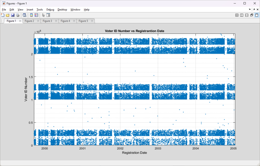
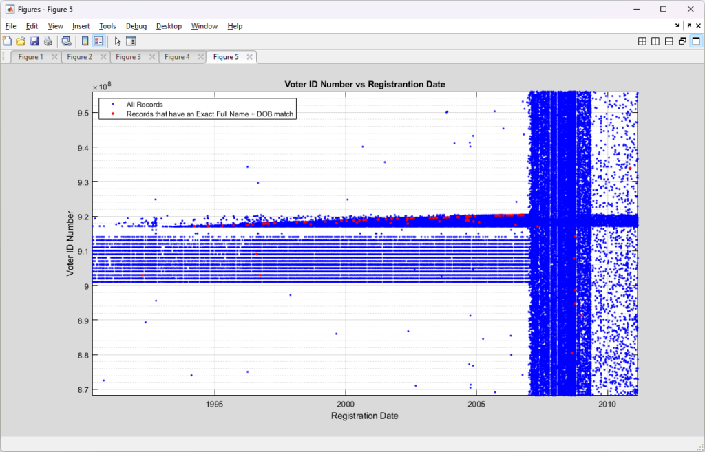
I previously had put together analysis that utilized the full name and date of birth information from the Virginia Registered Voter List (“RVL”) in order to look for duplicate registrations, either exact matches or by using a string distance measure (the Levenshtein distance) to accommodate for typos, abbreviations, and mis-spellings.
Just prior to the start of early voting in the 2024 November General Election, we were notified that the department of elections (“ELECT”) was removing the full date of birth from the data we purchase. This removal of the full date of birth increased the number of false positive in our duplication detection scripts. Our organization, as well as others, were ready to go to court to compel ELECT to reinstate the data. (Link to our notice of violation letter is here).
Happily, we ended up not having to go to court as ELECT decided to reinstate the data earlier this year (~May timeframe), which means we can resume our computation and detections of potentially duplicate entries again with much more reliable results. The results below mirror our previous analysis, but with the new updated data.
Using the latest Registered Voter List (RVL) and Voter History List (VHL) data purchased directly from the VA Department of Elections (ELECT) I wrote up an analysis script to check for potentially duplicated registrant records in the RVL and cross reference duplicate pairings with the VHL to identify potential duplicate votes. The details are summarized below.
Please note that I will not publish voter Personally Identifiable Information (PII) on this blog. I have substituted fictitious, but representative, PII information for all examples given below, and cryptographically hashed all voter information in the downloadable results file. I will make available the detailed information to those that have the authorization to receive and process voter data upon request (contact us).
Summary of Results:
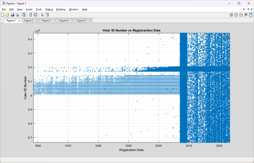
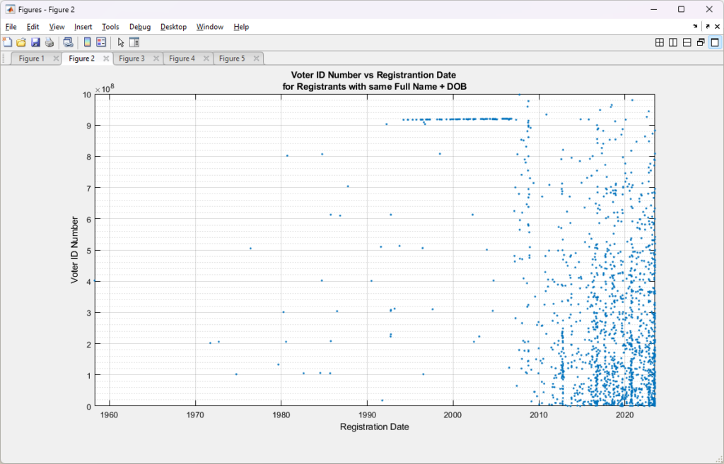
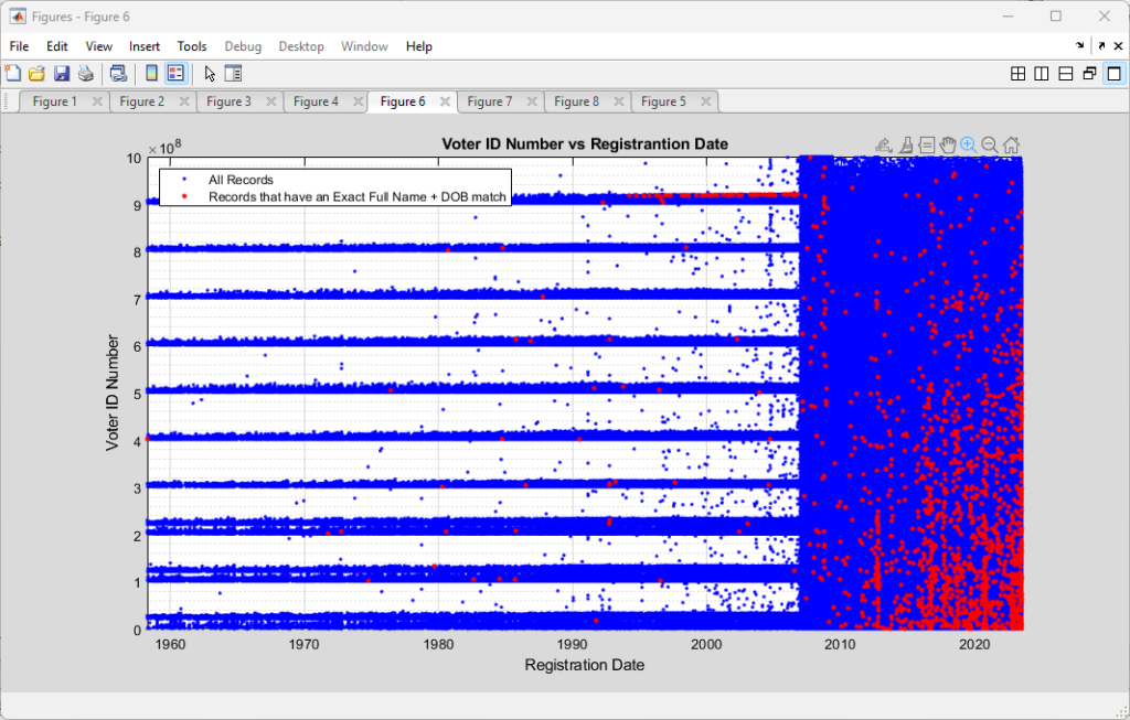
As a baseline, there were 5,514 (as compared to 6,464 in the previous May 27, 2023 posting) records for STATUS=’Active’ registrants that adhered to the definition of a “duplicate” when Social Security Number (SSN) is not available, as defined by the MOU between DMV and ELECT (section 7.3) of having the same First Name + Last Name + Full Date of Birth (DOB). It should be noted that most records held by DMV and ELECT have a SSN associated with them (or at least they should). SSN information is not distributed as part of the data purchased by us from ELECT, however, so this is the appropriate standard baseline for this work.
Upgrading our definition of a potential duplicate to [First + Middle + Last + Suffix + DOB] and using a LevenshteinDistance=0 (meaning an exact match) drops the number of potential duplicates to 1,062 (1,982 previously), with each identified registrant in a pair having an exactly matching string result and unique voter ID numbers.
According to my derivations and simulations that are described in detail here, we should only expect to see an average of 11 (+/- 3) potential duplicate pairs (a.k.a. “collisions”) at a distance of 0. This is over two orders of magnitude different than what we observe in the compiled results. Such a discrepancy deserves further investigation and verification.
Allowing for a single string difference by setting LevenshteinDistance<=1 increases the pool of potential duplicates to 4,572 (5,568 previously). While this relaxation of the filter does allow us to find certain issues (described below) it also increases our chances of finding false positives as well. The LD metric results should not be viewed as a final determination, but as simply a useful tool to make an initial pass through the data and find candidate matches that still require further review, verification and validation.
Increasing to LevenshteinDistance<=2 brings the number of potential duplicates up to 27,178 (32,610 previously). When we increase to LD <= 3 we get an explosion of 158,940 (183,130 previously) potential duplicates.
It should be noted that compared to our last full analysis (May 2023) the dept of elections has reduced the number of exact duplicates by about 45%, and by approximately 13-15% for the other inexact categories.
Method:
For every entry in the latest RVL, I performed a string distance comparison, based on Levenshtein distance, between every possible pair of strings of (FIRST NAME + MIDDLE NAME + LAST NAME + SUFFIX + FULL DOB). For the ~6M+ different RVL entries, we therefore need to compute ~3.8 x 10^13 different string comparisons, and each string comparison can require upwards of 75 x 75 individual character comparisons, meaning the total number of character operations is on the order of 202.5 Quadrillion, not including logging and I/O.
A distance of 0 indicates the strings being compared are identical, a distance of 1 indicates that there a single character can be changed, inserted or removed that would convert one string into the other. A distance of 2 indicates that 2 modifications are required, etc.
Example: The string pair of “ALISHA” –> “ALISHIA” has an LD of 1, corresponding to the addition of an “I” before the final “A”.
I aggregated all of the Levenshtein distance pairings that were less than or equal to 3 characters different in order to identify potential (key word) duplicated registrants, and additionally for each pairing looked at the voter history information for each registrant in the pair to determine if there was a potential (again … key word) for multiple ballots to be cast by the same person in any given election. As we allow for more characters to be different, we potentially are including many more likely false positive matches, even if we are catching more true positives.
For example: At a distance of 4 the strings of “Dave Joseph Smith M 10/01/1981” and “Tony Joseph Smith M 10/01/1981” at the same address would produce a potential match, but so would “Davey Joseph Smith M 10/01/1981” and “David Josiph Smith M 10/02/1981”. The first pair is more likely to be a false positive due to twins, while the second is more likely to be due to typo’s, mistakes, or use of nicknames and might warrant further investigation. A much stronger potential match would be something like “David Josiph Smith M 10/01/1981” and “David Joseph Smith M 10/01/1981”, with a distance of 1 at the same address. In an attempt to limit false positives, I have clamped the distance checks to <= 3 in this analysis.
Note that the Levenshtein distance measure is importantly able to identify potential insertions or deletions as well as character changes, which is an improvement over the Hamming distance measure. This is exampled by the following pairing: “David Joseph Smith M 10/01/1981” and “Dave Joseph Smith M 10/01/1981”. The change from “id” to “e” in the first name adds/subtracts a character making the rest of the characters in the remainder of the string shift position. A Levenshtein metric would correctly return a small distance of 2, whereas the hamming distance returns 27.
Also note that with the official records obtained from ELECT, and in accordance with the laws of VA, I do not have access to the social security number or drivers license numbers for each registration record, which would help in identifying and discriminating potential duplicate errors vs things like twins, etc. I only have the first name, middle name, last name, suffix, month of birth, day of birth, year of birth, gender, and address information that I can work with. I can therefore only take things so far before someone else (with investigative authority and ability to access those other fields) would need to step in and confirm and validate these findings.
Results:
The summary totals are as follows, with detailed examples.
DMV_ELECT MOU Standard
LD <= 0
LD <= 1
LD <= 2
LD <= 3
Number of Potential Duplicate Registrant Pairs
6,108
1,250
5,116
29,480
170,772
Number of Potential Duplicate Registrant Pairs (Active Only)
5,514
1,062
4,572
27,178
158,940
Number of Potential Duplicate Ballots
2,856
58
1,580
16,984
109,428
Number of Potential Duplicate Ballots (Active Only)
2,770
54
1,552
16,410
105,932
Examples of Types of Issues Observed:
NOTE THE BELOW INFORMATION HAS HAD THE VOTER PERSONALLY IDENTIFIABLE INFORMATION (“PII”) FICTIONALIZED. WHILE THESE ARE BASED ON REAL DATA TO ILLUSTRATE THE DIFFERENT TYPES OF OBSERVATIONS, THEY DO NOT REPRESENT REAL VOTER INFORMATION.
Example #1: The following set of records has the exact match (distance = 0) of full name and full birthdate (including year), but different address and different voter ID numbers AND there was a vote cast from each of those unique voter ID’s in the 2020 General Election. While it’s remotely possible that two individuals share the exact same name, month, day and year of birth … it is probabilistically unlikely (see here), and should warrant further scrutiny.
Voter Record A:
AMY BETH McVOTER 12/05/1970 F 12345 CITIZEN CT
Voter Record B:
AMY BETH McVOTER 12/05/1970 F 5678 McPUBLIC DR
Example #2: This set of records has a single character different (distance of 1) in their first name, but middle name, last name, birthdate and address are identical AND both records are associated with votes that were cast in the 2020, 2021, and 2022 November General Elections. While it is possible that this is a pair of 23 year old twins (with same middle names) that live together, it at least bears looking into.
Voter Record A:
TAYLOR DAVID VOTER 02/16/2000 M 6543 OVERLOOK AVE NW
Voter Record B:
DAYLOR DAVID VOTER 02/16/2000 M 6543 OVERLOOK AVE NW
Example #3: This set of records has two characters different (distance of 2) in their birthdate, but name and address are identical AND the birth years are too close together for a child/parent relationship, AND both records are associated with votes that were cast in the 2020 and 2022 November General Elections.
Voter Record A:
REGINA DESEREE MACGUFFIN 02/05/1973 F 123 POPE AVE
Voter Record B:
REGINA DESEREE MACGUFFIN 03/07/1973 F 123 POPE AVE
Example #4: This set of records has again a single character different (distance of 1) in the first name (but not the first letter this time) and the last name, birthdate and address are identical. There were also multiple votes cast in the 2019 and 2022 November General from these registrants.
Voter Record A:
EDGARD JOHNSON 10/19/1981 M 5498 PAGELAND BLVD
Voter Record B:
EDUARD JOHNSON 10/19/1981 M 5498 PAGELAND BLVD
Example #5: This set of records has two characters different (distance of 2) in the first and middle names and the last name, birthdate, gender and address are identical. There were also multiple votes cast in the 2021 and 2022 November General from these registrants. Again it is possible that these records represent a set of twins given the information that ELECT provides.
Voter Record A:
ALANA JAVETTE THOMPSON 01/01/2003 F 123 CHARITY LN
Voter Record B:
ALAYA YAVETTE THOMPSON 01/01/2003 F 123 CHARITY LN
Example #6: The following set of records has the exact match (Distance = 0) of full name and full birthdate (including year), and same address but different voter ID numbers. There was no duplicated votes in the same election detected between the two ID numbers.
Voter Record A:
JAMES TIBERIUS KIRK 03/22/2223 M 1701 Enterprise Bridge
Voter Record B:
JAMES TIBERIUS KIRK 03/22/2223 M 1701 Enterprise Bridge
Example #7: The following set of records has the exact match (distance = 0) of full name and full birthdate (including year), same address but different gender and voter ID numbers. There was no duplicated votes in the same election detected between the two ID numbers.
Voter Record A:
MAXWELL QUAID CLINGER 11/03/2004 M 4077 MASH DR
Voter Record B:
MAXWELL QUAID CLINGER 11/03/2004 U 4077 MASH DR
Example #8: The following set of records has a single punctuation character different, with the same address but different voter ID numbers. There was no duplicated votes in the same election detected between the two ID numbers.
Voter Record A:
JOHN JACOB JINGLHIEMER-SCHMIDT 06/29/1997 M 12345 JACOBS RD
Voter Record B:
JOHN JACOB JINGLHIEMER SCHMIDT 06/29/1997 M 12345 JACOBS RD
Results Dataset:
A full version of the aggregated excel data is provided below, however all voter information (ID, first name, middle name, last name, dob, gender, address) have been removed and replaced by a one-way hash number, with randomized salt, based on the voter [First Name, Middle Name, Last Name, Suffix, and DOB]. The full file with specific voter information can be provided to parties authorized by ELECT to receive and process voter information, Election Officials, or Law Enforcement upon request.
Recently I was made aware of the work Ed Solomon had been doing with data from the 2020 Colorado Cast Vote Records (CVRs), and I’ve taken some time to replicate and validate some of his data observations. I don’t always agree with Ed, but I wanted to take some time and verify the facts of the matter for myself.
For background, CVRs are machine logs of the way the tabulators process the “cast” ballots. You can think of them as equivalent to your bank statement showing all of the recorded transactions for each ballot scanned. They are required to be producible by ballot electronic tabulation systems, and are used as part of official forensic audits and documentation. They do not have any personal information and simply operate on the content of individual ballots as they are processed.
There are 2 specific items that need to be validated here:
Odd statistics associated with statewide ballot measures in Arapahoe County as compared to other counties. Specifically, there were two statewide ballot measures (one dealing with taxes, and another on abortion) that one would expect to show a significant partisan split, and we in fact do see such a split in neighboring El Paso and Adams counties. However, the ballot measures do not show the partisan split in Arapahoe County.
The difference is not just that the partisan split is muted or reduced, it is a night and day difference. In Arapahoe county there is almost no statistical difference between Trump and Biden voters on the ballot measures, but there is an obvious and clear difference on the same ballot measures in neighboring Adams and El Paso counties.
Why is this important? It raises questions as to the veracity of the election counts, data handling practices, and the ability to use CVRs for their intended forensic purpose.
The fact that the Arapahoe County CVR data was changed on the official county website without any notification or explanation around Feb 2025. The internal composition of ballots was changed in the data and “scrambled” by Arapahoe county … with the new version of the CVR files no longer showing the inconsistency from #1.
As CVRs are official records that are used for legal purposes such as audits etc., they should never be “quietly” changed or modified retroactively. A full and transparent explanation of the issues and steps made to remedy should accompany any updates for official documents such as CVRs.
This change took place years after the CVR was originally produced, and after Ed Solomon had used this particular CVR as part of his supporting documentation in an election case (Thompson vs Secretary of State NV) in Nevada.
The county was fully aware of the use of these records in the Nevada case.
The county CVRs had already been used in a previous audit of the 2020 election, where ballots from a specific tabulator and batch were pulled and compared to the cast vote record for accuracy. (see here, and here)
After Ed and Mark noticed the retroactive modifications and started asking questions, the County released a statement explaining that they were contacted by a researcher about potential issues with their CVR regarding “redaction” and privacy concerns.
However, the county statement gives an incompatible date for when the documents were “corrected”, according to the file timestamps and internet archive logs. The statement claims April 2nd 2025, whereas the contents of the uploaded file show Feb 20th 2025 as the file modification date.
The counties explanation does not comport with the observation of the scrambling of internal contents of official ballots. Its not just that the ordering of ballots was randomized to assuage privacy concerns, but that the actual records of votes cast were being swapped between ballots.
At BEST this shows a woeful lack of transparency and procedural safeguards by the county.
At WORST this has the appearance of being intentional tampering with official records.
I can independently replicate and validate both of these data observations. There does seem to be an issue with the ballot measures in the original Arapahoe County CVR data, and that data has been retroactively modified by the county in such a way as to scramble the information associated with votes cast.
Note that Ed Solomon, Draza Smith, Jeff O’Donnell (a.k.a. “The Lone Raccoon”), Mark Cook, MadLiberals, and others all provided data and pointers to the original documents and URLs in question, as well as their own analysis on the X.com platform.
The original data is also still available on the Arapahoe County website, but one needs to do some creative sleuthing via the wayback machine and looking at the URL links in order to get to it, as was done by Mark Cook. (see: here and here)
The original data from the 2020 CVR data had also been collected and collated by Jeff O’Donnell on his https://votedatabase.com (formerly ordros.com) site, which I archived and versioned in Sept of 2022. I can confirm that the original file matches the files in the votedatabase archive, as well as the current votedatabase site. I used additional files from votedatabase archive for neighboring Adams and El Paso counties as a source for the rest of this work, as I could not find corresponding links to CVR downloads on the Adams or El Paso county websites.
Ed’s original observation was that the two ballot measures that *should* be partisan split were not when looking at the original 2020 CVR Arapahoe County data. He used this observation as supporting evidence showing inconsistencies and irregularities in 2020 election data in an court case (Thompson vs Secretary of State NV) he was providing analysis for in Nevada. All of his analysis and the original file have therefore been previously submitted to the court.
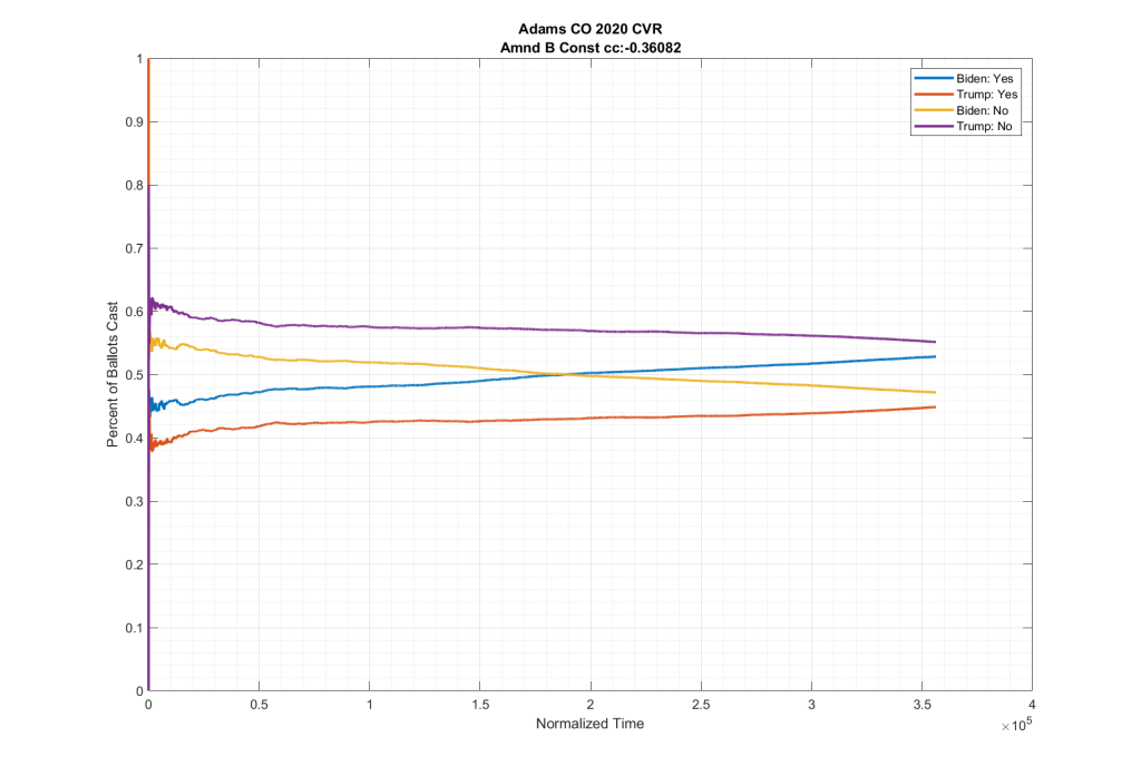
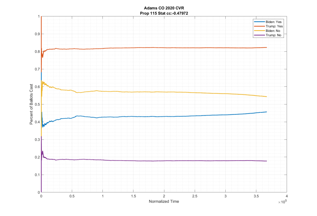
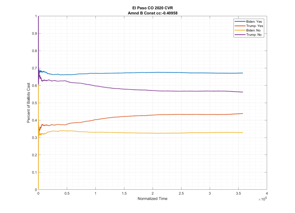
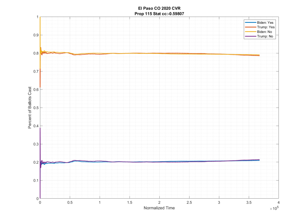
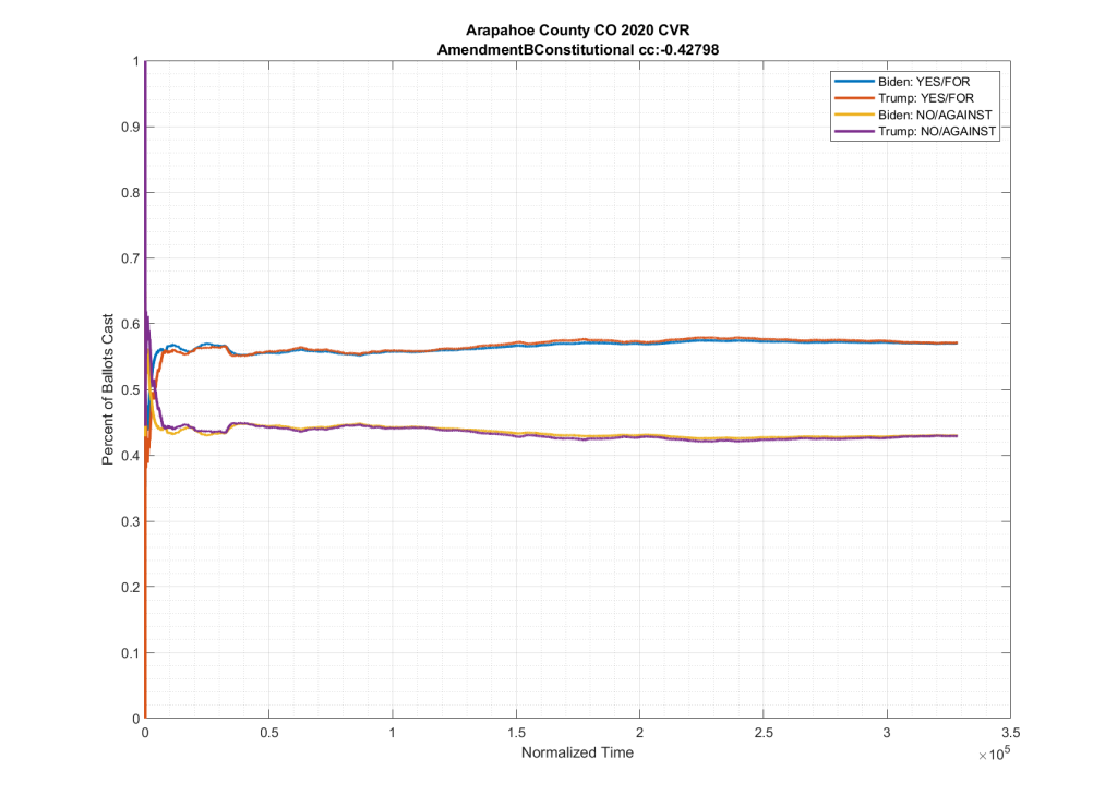
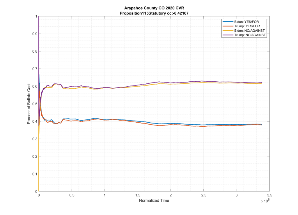
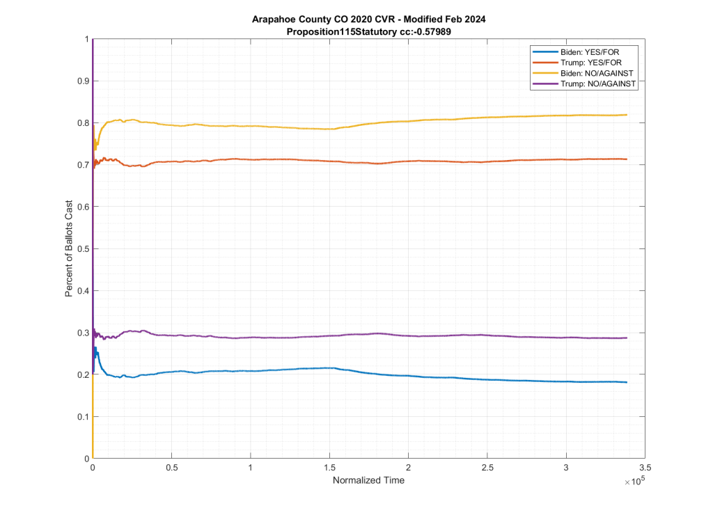
Amendment B was a repeal of the “Gallagher Amendment” dealing with property tax rates and was expected to have a highly partisan split. Likewise Proposition 115 dealt with abortion and was also expected to have highly partisan split.
If we look at the plots of the ballots cast for these two ballot measures, but we condition them on if the person voted for Trump or Biden at the top of the ticket we do see in neighboring counties such as El Paso and Adams counties this partisan split, as shown below. Note the significant spread between the Biden/No (Yellow) & Trump/No (Purple), as well as between the Biden/Yes (Blue) & Trump/Yes (Red).
As can be seen in the plots above from Adams and El Paso counties, there is a significant partisan split in these two down-ballot races when conditioned on how the top of the ticket votes. However this seems to vanish when looking at Arapahoe County, with the Biden/No (Yellow) & Trump/No (Purple) and the Biden/Yes (Blue) & Trump/Yes (Red) stacking almost completely on top of one another.
It can be clearly seen in the plots that the partisan split that was present in the other counties results seems to have completely vanished in Arapahoe.
I will note that the partisan split seems to be missing from almost all down-ballot races that I looked at, not just these two, although these were the ones specifically called out by Ed. This is an important point that I will come back to in a minute.
… And now to item # 2:
Ed’s original observation was submitted as part of his case in Nevada. At one point he and Mark Cook attempted to make a live stream video showing how people could recreate the observations starting from the source documents on the Arapahoe County website, which is when he and Mark realized that the original CVR file on the county website had been quietly replaced with a new file that had its contents scrambled and the results no longer showed the observed pattern.
Note that a CVR file is a legally required forensic record. It is the equivalent of a bank transaction log, and should almost never have its contents manipulated. If an error is discovered, and a correction does need to be issued, then a new file with the corrections should be published along side the original with a clear and prominent explanation and notification of the change. In this case, however, the County simply replaced the link to the original file with the new file with no explanation and no notice.
It was only after this was discovered, and after Ed started making phone calls to the County and bringing up the issue with the Judge in his Nevada case, that Arapahoe County belabouredly published an admission that they had adjusted the file. Their excuse for the modification was that they were made aware of a mistake with their “redaction” of data in the original publication, and were worried about individual privacy.
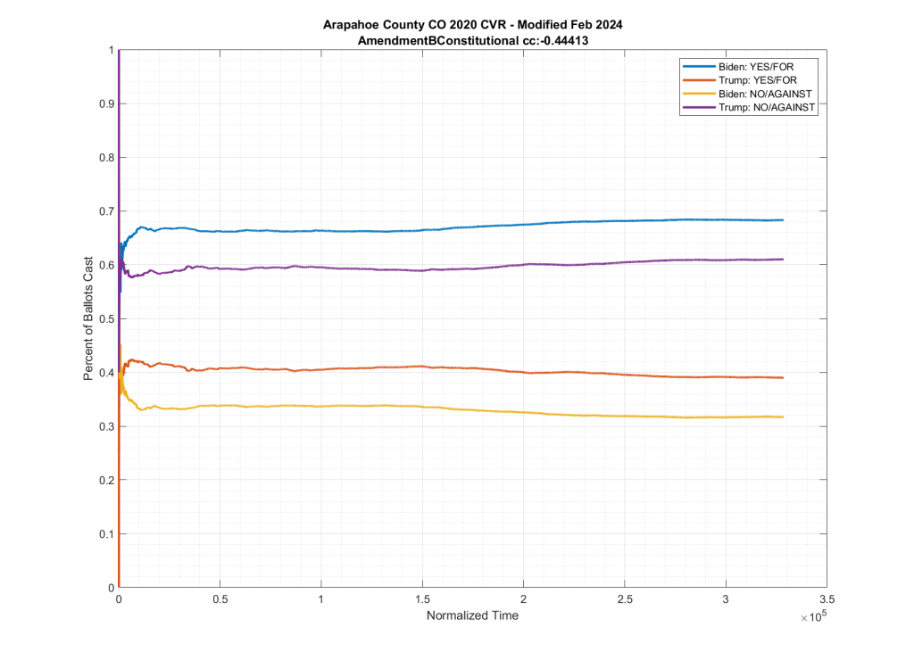
The (new) altered file did have 16 specific ballots that had their down-ballot races zeroed out, and was missing the “CountingGroup” metadata column. However, the file didn’t just have a small number of ballots (16) down-ballot information omitted, the internal contents on ALL ballots were also completely scrambled, with the top-of-the-ticket entries for President and Senate and metadata columns being completely reordered from all of the down-ballot information. This split-scrambling also also “fixed” the observed issues with Amendment B and Proposition 115, as can be seen below, where there is now a distinct partisan split between the data trends.
This kicked off multiple efforts to reverse engineer the actual changes that were performed on the CVR data by Arapahoe county, by myself and multiple others. Jeff O’Donnell and MadLiberals on X made the observation of the split reordering. I was able to verify this and remove the split-shuffling, exposing the fact that there were 16 ballots that also had all of their down ballot information zeroed out. There were a total of 432 down ballot votes that were removed from 16 specific ballots, followed by ALL of the President and Senate votes for ALL ballots being scrambled in relation to their down-ballot races.
Back to the point I made before above … the “scrambling” of the new file does seem to have “fixed” the expected partisan nature of most of the down-ballot races, so it is not unreasonable to think that this was actually a “fix” for a processing error on the original CVR file. That being said, the original (assumed incorrect) CVR was used in an audit process of two down-ballot races (linked above). Why did they not catch this issue years earlier during the audit? And why did they make the change to files, under the pretense of privacy issues, without announcing and documenting the errors?
Conclusion:
I can verify the two main data issues documented by Ed Solomon on the Arapahoe County 2020 CVR data.
The original data file had significant issues with down-ballot races not showing the expected partisan splits.
Arapahoe county did “quietly” revise the data without explanation until it was discovered by Ed and Mark, and then when pushed, only acknowledged that there was an issue with redactions and data privacy concerns.
The fact that the modification did correct the expected partisan split for ALL down-ballot races lends some credence to the assertion that they were correcting an error/issue with the original CVR file, however it does not excuse the fact that they performed this correction without notice or explanation. It also does not explain how their 2020 audit was able to use the incorrect original CVR files and not catch any of these issues.
The CVR files are intended to be official forensic records. If they are subject to manipulation and “adjustments” without transparency then that brings into question the validity of those files as forensic devices in the first place.
Corrections:
(5/28/2025) Typo correction in that the original posting of this article had “April 2 2024” as the data the Arapahoe county statement said they changed the CVR. That was corrected to be “April 2 2025”.
(5/28/2025) I had the wrong reference for the associated case in NV. I had originally posted that the case was the “Gilbert” case. It is actually “Thompson vs State”. Links have been updated accordingly.
Using data published by the VA Department of Elections (“ELECT”), we plotted the Ballot Invalidation Rate (BIR) vs. the % of vote share for the winner in order to attempt to determine if “Differential Invalidation” of ballots occurred in the 2024 VA General Election. The plotted data appears to show differential invalidation and suggests that there are underlying issues that should be investigated and addressed, including data reliability and consistency issues where the number of reported total votes cast is greater than the number of reported ballots cast for some localities.
Details
“Differential invalidation” takes place when the ballots of one candidate or position are invalidated at a higher rate than for other candidates or positions. Note that differential invalidation does not directly indicate any sort of fraud. It is however indicative of an unfairness or inequality in the rate of incomplete or invalid ballots conditioned on candidate choice. While it could be caused by fraud or malfeasance, it could also be caused by confusing ballot layout, poor procedural controls and uniformity, under-voting (not choosing a candidate) by the voter, or other compounding factors, etc. (ref: [1] ch. 6)
The Free and Fair Hypothesis
In a democratic election, each persons vote counts the same. There are other requirements, but this is a necessary condition. In the presense of invalidation, the free and fair hypothesis reduces to each person’s vote having the same probability of being invalidated as any other persons ballot. From a statistical standpoint, this means that the invalidation must be independent of the candidate chosen on the ballot (or of the person voting) [ref: 1, pg. 132]
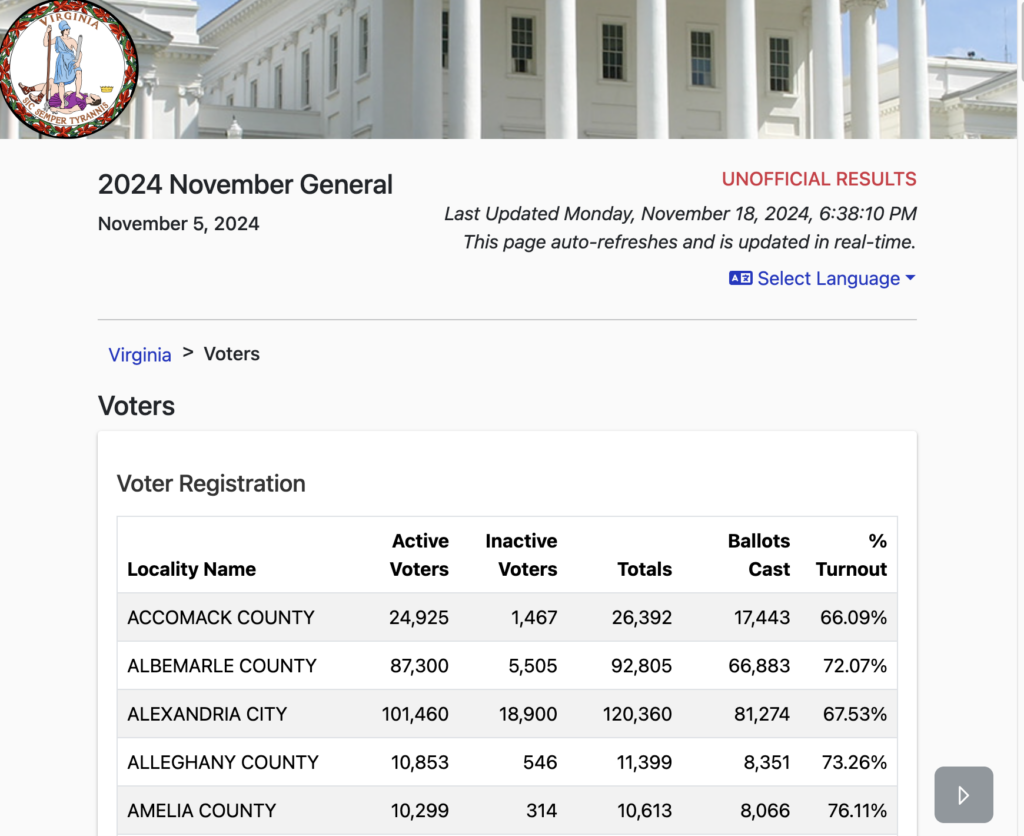
The data used for this analysis was the “unofficial” election results (the certified results are not yet published), and comes directly from the VA Dept of Elections. The data was downloaded on Nov 18th at 4:34 pm. We purposefully waited to perform this analysis until after the localities had completed their canvass operations, and for the data feeds on the VA Department of Elections (“ELECT”) website to mostly stabilize. The actual certified results will not be available until at least Dec 2 after the State Electoral Board meets to finalize the certification. We will revisit this analysis at that time.
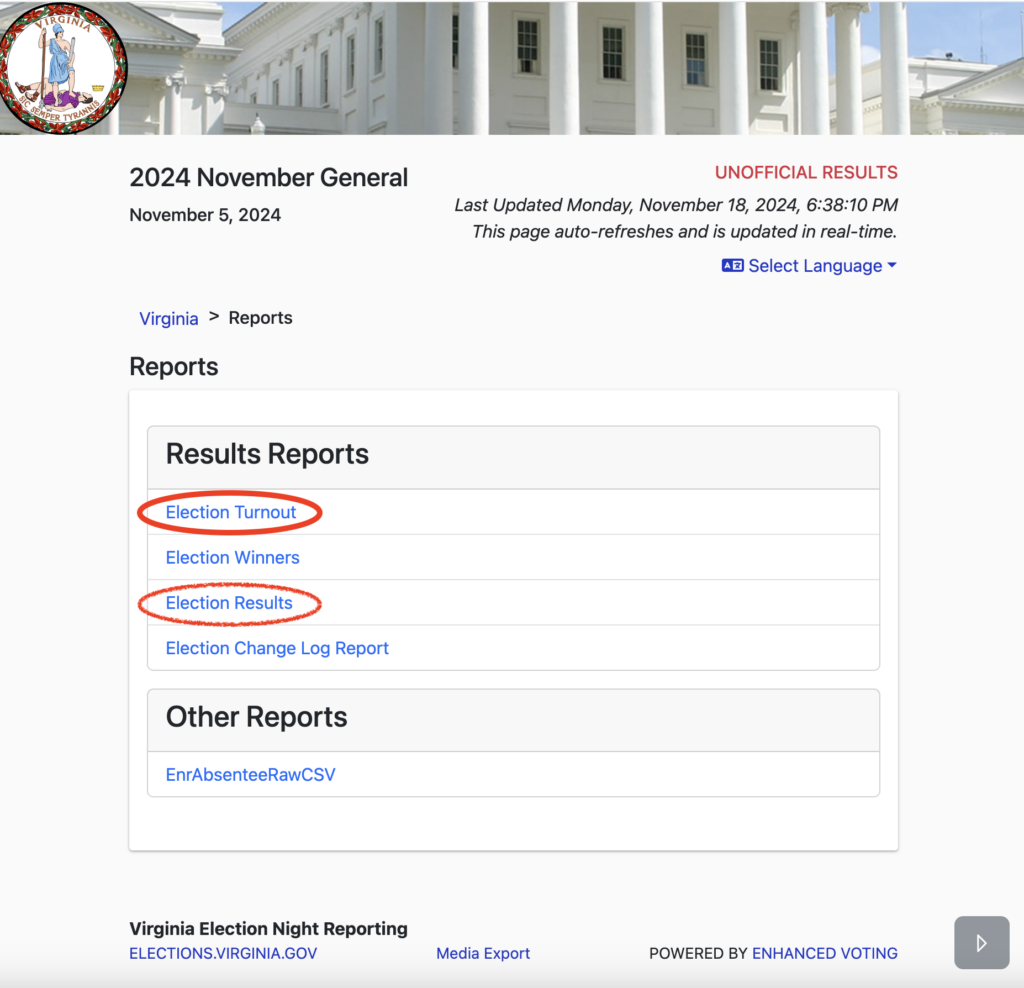
Figure 2: Listing of the link for report CSV files as appeared on the VA Dept of Elections Website on Nov 18 16:34:00 EST at https://enr.elections.virginia.gov/results/public/Virginia/elections/2024NovemberGeneral/reports. Note that additional CSV files for “Election Winners”, “Election Change Log Report”, “EnrAbsenteeRawCSV”, as well as a complete JSON listing under the “Media Export” link at the bottom of the page.
With this dataset in hand we can know how many ballots were cast, as well as how many votes were counted for each candidate in each race in each locality (at least as reported by the state). For a given race, we can then compute the number of incomplete or invalid ballots by subtracting the total number of votes recorded for that race in the locality from the total number of reported ballots cast.
In accordance with the techniques presented in [1] and [2], we computed the plots of the Invalidation Rate vs the Percent Vote Share for the Winner in an attempt to observe if there looks to be any evidence of Differential Invalidation ([1], ch 6). This is similar to the techniques presented in [2], which we have used previously to produce election fingerprint that plotted the 2D histograms of the vote share for the winner vs the turnout percentage. (The 2024 versions are coming, just not ready yet.)
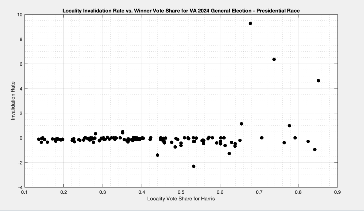
Each dot in Figure 3 below is representing the ballots from a specific locality. The x axis is the percent vote share for the winner (Harris), and the y axis is the ballot invalidation rate, and is computed as 100 – 100 * Nvotes / Nballots.
Figure 3: Plot of the Invalidation rate vs the % of vote share for the winner in each locality in the 20204 VA General Election for President.
A few things are immediately apparent from the plot in Figure 3:
There is clearly a distinction in the invalidation rate between localities that had low vote share and high vote share for harris.
The data for localities where Harris had low vote share do not have a large distribution of invalidation rates, whereas the high vote share localities do.
There are a number of localities that are reporting negative invalidation rates. How is this possible, you ask? Well there are a number of localities in the CSV data that have higher vote totals than the corresponding reported number of total ballots cast in the locality.
This implies that there is something significantly wrong in the data and reporting tools or procedures used by ELECT, as all of this data was pulled nearly simultaneously and therefore the data should be at least self-consistent. While we understand that this is still unofficial data and that new updates may occur over time, at any given point in time the data should at least be self-consistent.
Note that there are still a few localities that have not yet had their vote totals reflected in the CSV files from ELECT. Those localities were omitted from this analysis. The combined information from all of the data source files that was used to generate this plot is available below.
In conclusion there does appear to be some indications that differential invalidation occurred in the 2024 VA General Election for President. Due to data inconsistencies and the fact that this data is still officially “unofficial” it is hard to make any definitive conclusions, but these results are suggestive of the existence of multiple underlying issues that need to be examined, understood and/or resolved. We can definitively say, however, that this is yet another example of the data streams from ELECT lacking self-consistency, which is a big problem in and of itself.
References
[1] Forsberg, O.J. (2020). Understanding Elections through Statistics: Polling, Prediction, and Testing (1st ed.). Chapman and Hall/CRC. https://doi.org/10.1201/9781003019695
[2] Klimek, Peter & Yegorov, Yuri & Hanel, Rudolf & Thurner, Stefan. (2012). Statistical Detection of Systematic Election Irregularities. Proceedings of the National Academy of Sciences of the United States of America. 109. 16469-73. https://doi.org/10.1073/pnas.1210722109.
EPEC has compared the changes to two purchased full versions of the VA Registered Voter List (RVL) to the content of the Monthly Update Service (MUS) data covering the same temporal period. Of the ID numbers that were added to the RVL, 3,613 (or 1.0589% of total additions) never appear anywhere in the MUS files covering the same temporal period. Of the ID numbers that were removed from the RVL, 3,355 (or 2.4096% total removals) never appear anywhere in the MUS files covering the same temporal period.
Since mid 2023 EPEC has been purchasing, processing and archiving copies of both the full Registered Voter List (RVL) and the Monthly Update Service (MUS) files which gives the UPDATE, ADD or CANCEL transactions to the voter list throughout the year.
Once a baseline RVL is established, the MUS files can be used to update that baseline in order to keep the list current. That should be all one needs to keep an accurate dataset of the registered voter list using monthly updates … except there is a catch … the MUS for some reason doesn’t quite capture all of the changes that are occurring in the voter list. In fact, we see about 1-2.5% of the ADD or CANCEL transactions between each RVL snapshot are not reflected by any corresponding entries in the MUS.
All of the changes that are made between two different RVL baseline snapshots should be able to be observed in the corresponding MUS files that cover the same time period, and vice versa. The MUS has transaction logs accounting for new registrants, for registrants who move, for removing deceased individuals, for individuals that have had a change in their felon status, for individuals who are determined non-citizen, for administrative updates and correction, etc. So, in theory, it should be able to be a complete record. However, over the course of working with the VA data files, every so often we have noticed that some transactions seem to be unaccounted for. Therefore, once we had enough data compiled, we decided to test just how well the MUS data actually explains the changes we see between between two baseline RVL files.
Method:
For this experiment, we used full RVL snapshots purchased from VA Department of Elections (ELECT) on 2023-06-30 and 2024-08-29, and all of the monthly MUS distributions covering the entire time period in between.
Using the voter ID number field that is present in all datasets, we first determine which ID numbers were added to the 2024 RVL dataset, and which ID numbers were deleted from the 2023 RVL data. We then checked to see how many of those ID numbers appear in any of the MUS data files, for any reason.
Note that this data was processed statewide, such that registrants moving between localities within the state should not affect the total number of computed additions or removals, as the ID numbers should still be present in the datasets, although corresponding locality information may have changed.
Results:
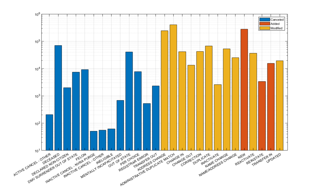
The breakdown of the number of changes that were present in the MUS file over the time period of the RVL snapshots (2023-06-30 through 2024-08-29) is given in Figure 1 below. The MUS data was deduplicated and truncated to only consider transactions with TRANSACTION date information between the dates associated with the RVL datasets. The bars in Figure 1 are logarithmically scaled in the y-axis, with the x-axis representing the NVRAReasonCode given for each transaction in the MUS. The bars are color coded by transaction type. As there are duplicates and oversampling within the collection of MUS files, only the latest transactions for each uniquely identified ID number was utilized to generate the plot. As can be seen from the various categories along the x-axis of this plot, the data in the MUS logs should be sufficient to capture all of the transactions with the RVL.
Figure 1: Breakdown of MUS transactions between 2023-06-30 and 2024-08-29
Direct Inspection of the RVL Snapshots:
Performing a simple set-difference between the elements of the unique ID numbers present in the 2023-06-30 RVL data vs the 2024-08-29 RVL data shows that there were 341,191 unique ID’s added, and 139,232 removed between the two datasets.
Of the ID numbers that were ADDED between the raw RVL snapshots, 3,613 (or 1.0589%) never appear anywhere in the MUS files covering the same temporal period.
Of the 3,613 ID numbers that were ADDED between the raw RVL snapshots, and that don’t appear in the MUS record, 537 (or 14.863%) have at least one entry in the Voter History List (VHL) data the EPEC has been collecting and archiving.
Of the ID numbers that were REMOVED between the raw RVL snapshots, 3,355 (or 2.4096%) never appear anywhere in the MUS files covering the same temporal period.
Of the 3,355 ID numbers that were REMOVED between the raw RVL snapshots, and that don’t appear in the MUS record, 2,011 (or 59.94%) have at least one entry in the VHL data the EPEC has been collecting and archiving.
Using the MUS-Adjusted RVL baseline
If we ignore the 2024-08-29 dataset, and instead directly apply the transactions in the MUS datafiles to the 2023-06-30 dataset in order to create a new RVL list, we would end up with 342,888 Additions, and 137,849 removals respectively to unique voter ID numbers. We see 1,697 more (342,888-341,191=1697) additions when trying to directly apply the MUS than when directly comparing RVL snapshots, and 1,383 less (139,232-137,849=1393) removals. Keep in mind these discrepancies are in addition to the 3,613 and 3,355 discrepancies using the RVL snapshot baselines, as the ID numbers in each set are unique. So the total number of discrepancies is 3,613 + 3,355 + 1,697 + 1,383 = 10,048 records.
We do not understand yet the origin of these discrepancies, it could be a coding error on the part of the developers of the VERIS system, or it could be that there is a category of data adjustments that is not adequately reflected in the RVL or MUS data products. The RVL snapshots are supposed to be the authoritative record of the voter registration data, and the MUS data updates are supposed to capture all of the transactional changes to said registration records.
Regardless of the cause of the discrepancy, the fact remains that there are a small number of transactions and changes to the voter record that are unobservable. They are, in effect, “dark” transactions in the voter registration data that cannot be observed, validated or verified.
Building off of our previous work on computing the string distance between all possible pairs of registered voter records in a single state in order to identify potential matches, we’ve updated the code to allow for cross state comparisons. The first states that we ran this on was VA and FL, using the dataset produced by the FL Department of Elections on 05-07-2024, and the dataset from the VA department of elections dated 05-01-2024. There were a total of 2,502 records that matched our constraints between the FL and VA datasets, as detailed below.
Note: All examples of data records given in this writeup have been fictionalized to protect registered voter identities from being published on this website, and only serve as illustrative examples representative of the nature of properties and characteristics discussed. Law enforcement, election or other gov officials, or individuals otherwise authorized to receive and handle voter data as per VA law and the VA Department of Elections are welcome to contact us for specific details and further information.
Each dataset had the First Name, Middle Initial, Last Name, Suffix, Gender, and Year, Month and Day of Birth concatenated into strings that were then compared against each other using the Levenshtein String Distance measure as an initial filtering method to determine potential matches.
Additionally, for each pair we computed the minimum string distance measure between all of the four possible permutations of pairings between the Primary and Mailing addresses in each record between the states. We required that this minimum distance for a set of registration entries be less than or equal to 12 characters. The choice of the value of twelve was empirically determined after review of the data, as it is loose enough to allow for common variations in address presentation while not being so loose as to be overwhelmed with false positive.
We additionally filtered these findings for only those pairings that were of ACTIVE registrations in both datasets AND where the year, month and day of birth were exact matches.
In summary the 2,502 matches were generated according to the following constraints:
Only applied to ACTIVE voter registrations
Required completed DOB (year, month and day) to exactly match
Required [First Name + Middle Initial + Last Name + Suffix + Gender + DOB] strings to be similar to within <=2 characters
Required that the minimum distance between any pairwise combination of the Primary or Mailing address between the records be less than or equal to 12 characters.
It should be noted that it is readily apparent from reviewing the potential matched records that the majority of these matches look to have originated in FL and then were subsequently moved to VA, but the FL record remained listed as active.
Category 1 Matches:
There were 698 matches in Category 1: where the Levenshtein distance measure for the name and DOB was equal to 0 (exact match) and the minimum address distance was also 0 (also an exact match). Examples in this category are exact matches for every considered field. An example is given below.
FL Active Registration Record: SOUXIEE Q SMITH F 08/19/1968 1267 SLEEPY SONG PL SPRINGFIELD VA 22150
VA Active Registration Record: SOUXIEE Q SMITH F 08/19/1968 1267 SLEEPY SONG PL SPRINGFIELD VA 22150
Category 2 Matches:
There were 1,533 matches in Category 2: where the Levenshtein distance measure for the name and DOB was equal to 0 (exact match) and the minimum address distance was greater than 0, but less than or equal to 12. Examples in this category commonly have differences in how the zip code, apartment numbers or state code is presented in either the Primary or Mailing address strings. An example is given below.
FL Active Registration Record: SOUXIEE Q SMITH F 08/19/1968 1267 SLEEPY SONG PLACE SPRINGFIELD VA 22150
VA Active Registration Record: SOUXIEE Q SMITH F 08/19/1968 1267 SLEEPY SONG PL SPRINGFIELD VA 221504259
Category 3 Matches:
There were 44 matches in Category 3: where the Levenshtein distance measure for the name and DOB was equal to 1 and the minimum address distance was equal 0 (exact match). Examples in this category are most often due to hyphenation or misspellings in the name, or a change in Gender (i.e. from “M”->”U”). An example is given below.
FL Active Registration Record: BENNIE DAS M 05/14/1945 12345 PEPPERMINT PATTY CREST APT 1000 ASHBURN VA 201475724
VA Active Registration Record: BENNEE DAS M 05/14/1945 12345 PEPPERMINT PATTY CREST APT 1000 ASHBURN VA 201475724
Category 4 Matches:
There were 140 matches in Category 4: where the Levenshtein distance measure for the name and DOB was equal to 1 and the minimum address distance was greater than 0, but less than or equal to 12. Examples in this category are most often due to hyphenation or misspellings in the name, or a change in Gender (i.e. from “M”->”U”), as well as small differences in how the addresses are presented. An example is given below.
FL Active Registration Record: BENNIE DAS M 05/14/1945 1267 SLEEPY SONG PLACE SPRINGFIELD VA 22150
VA Active Registration Record: BENNEE DAS M 05/14/1945 1267 SLEEPY SONG PL SPRINGFIELD VA 221504259
Category 5 Matches:
There were 19 matches in Category 5: where the Levenshtein sistance measure for the name and DOB was equal to 2 and the minimum address distance was equal 0 (exact match). Examples in this category are most often due to a middle name/initial being present in one record and not being present in the other. An example is given below.
FL Active Registration Record: BENNIE DAS M 05/14/1945 12345 PEPPERMINT PATTY CREST APT 1000 ASHBURN VA 201475724
VA Active Registration Record: BENNIE C DAS M 05/14/1945 12345 PEPPERMINT PATTY CREST APT 1000 ASHBURN VA 201475724
Category 6 Matches:
There were 68 matches in Category 3: where the Levenshtein Distance measure was equal to 1 and the minimum address distance was greater than 0, but less than or equal to 12. Examples in this category are most often due to a middle name/initial being present in one record and not being present in the other, as well as small differences in how the addresses are presented. An example is given below.
FL Active Registration Record: BENNIE C DAS M 05/14/1945 1267 SLEEPY SONG PLACE SPRINGFIELD VA 22150
VA Active Registration Record: BENNIE DAS M 05/14/1945 1267 SLEEPY SONG PL SPRINGFIELD VA 221504259
Table of Results by VA Locality:
Row Labels
LD=0, AD=0
LD=0, 0<AD<=12
LD=1, AD=0
LD=1, 0<AD<=12
LD=2, AD=0
LD=2, 0<AD<=12
ACCOMACK COUNTY
3
8
1
1
0
0
ALBEMARLE COUNTY
13
24
0
1
0
0
ALEXANDRIA CITY
15
52
1
6
1
1
ALLEGHANY COUNTY
1
3
0
1
0
0
AMELIA COUNTY
2
2
0
0
0
0
AMHERST COUNTY
3
2
0
0
0
0
APPOMATTOX COUNTY
5
0
0
0
1
0
ARLINGTON COUNTY
27
53
2
8
2
6
AUGUSTA COUNTY
3
8
0
1
1
0
BEDFORD COUNTY
4
15
0
1
0
0
BOTETOURT COUNTY
7
2
0
0
0
0
BRISTOL CITY
3
2
0
0
0
0
BRUNSWICK COUNTY
1
2
0
0
0
0
BUCHANAN COUNTY
1
0
0
0
0
0
BUCKINGHAM COUNTY
0
1
0
0
0
0
CAMPBELL COUNTY
2
3
1
1
0
0
CAROLINE COUNTY
0
2
0
0
0
0
CARROLL COUNTY
1
6
0
1
0
0
CHARLOTTE COUNTY
1
4
0
0
0
0
CHARLOTTESVILLE CITY
4
6
0
0
0
1
CHESAPEAKE CITY
27
87
4
13
1
4
CHESTERFIELD COUNTY
28
49
2
5
0
3
CLARKE COUNTY
0
2
0
0
0
0
COLONIAL HEIGHTS CITY
0
1
1
0
0
0
CRAIG COUNTY
2
1
0
0
0
0
CULPEPER COUNTY
6
8
0
0
0
0
CUMBERLAND COUNTY
2
0
0
0
0
0
DANVILLE CITY
2
1
0
0
0
0
DICKENSON COUNTY
1
3
0
0
0
0
DINWIDDIE COUNTY
0
3
0
1
0
0
ESSEX COUNTY
2
0
0
0
0
0
FAIRFAX CITY
3
6
0
0
0
0
FAIRFAX COUNTY
108
259
7
14
4
15
FALLS CHURCH CITY
2
2
0
0
0
1
FAUQUIER COUNTY
4
14
1
0
0
0
FLOYD COUNTY
1
1
1
0
0
0
FLUVANNA COUNTY
2
3
0
2
0
0
FRANKLIN CITY
3
1
0
0
0
0
FRANKLIN COUNTY
5
6
0
1
0
1
FREDERICK COUNTY
10
9
0
2
0
0
FREDERICKSBURG CITY
1
7
0
0
0
0
GALAX CITY
2
0
0
0
0
0
GILES COUNTY
0
0
0
1
0
0
GLOUCESTER COUNTY
6
17
0
1
1
0
GOOCHLAND COUNTY
2
2
1
0
1
0
GRAYSON COUNTY
1
3
0
1
0
0
GREENE COUNTY
0
5
0
0
0
0
HALIFAX COUNTY
1
2
0
1
0
0
HAMPTON CITY
10
16
0
6
0
0
HANOVER COUNTY
2
6
1
2
1
0
HARRISONBURG CITY
1
6
0
1
0
0
HENRICO COUNTY
24
33
0
3
0
1
HENRY COUNTY
3
5
0
1
0
0
ISLE OF WIGHT COUNTY
4
13
0
1
0
2
JAMES CITY COUNTY
23
25
1
1
0
0
KING GEORGE COUNTY
2
4
1
0
0
1
KING WILLIAM COUNTY
2
0
0
0
0
0
LANCASTER COUNTY
2
1
1
0
0
1
LEE COUNTY
3
1
0
0
0
0
LEXINGTON CITY
0
2
0
0
0
0
LOUDOUN COUNTY
29
73
1
1
2
2
LOUISA COUNTY
5
2
0
0
0
0
LYNCHBURG CITY
6
15
0
2
0
0
MADISON COUNTY
2
0
0
0
0
0
MANASSAS CITY
3
0
0
0
0
0
MANASSAS PARK CITY
1
0
0
0
0
0
MARTINSVILLE CITY
2
1
0
0
0
0
MATHEWS COUNTY
0
3
0
0
0
0
MECKLENBURG COUNTY
3
2
0
0
0
0
MIDDLESEX COUNTY
0
4
0
1
0
0
MONTGOMERY COUNTY
6
11
1
1
0
0
NELSON COUNTY
1
2
0
1
0
0
NEW KENT COUNTY
0
6
0
0
0
0
NEWPORT NEWS CITY
8
17
0
1
0
2
NORFOLK CITY
14
58
0
11
0
1
NORTHUMBERLAND COUNTY
2
1
1
0
0
0
NOTTOWAY COUNTY
0
1
0
0
0
0
ORANGE COUNTY
5
6
1
0
0
0
PAGE COUNTY
1
2
0
0
0
0
PATRICK COUNTY
0
2
0
0
0
0
PETERSBURG CITY
2
1
0
0
0
0
PITTSYLVANIA COUNTY
3
7
0
1
0
0
POQUOSON CITY
1
0
0
0
0
0
PORTSMOUTH CITY
5
9
1
1
0
0
POWHATAN COUNTY
2
2
0
1
0
0
PRINCE EDWARD COUNTY
0
2
0
0
0
0
PRINCE GEORGE COUNTY
1
1
1
1
0
1
PRINCE WILLIAM COUNTY
40
83
2
11
3
3
PULASKI COUNTY
2
2
0
0
0
0
RADFORD CITY
0
2
0
0
0
0
RAPPAHANNOCK COUNTY
0
2
1
0
0
0
RICHMOND CITY
12
29
1
3
0
0
ROANOKE CITY
14
12
1
2
0
0
ROANOKE COUNTY
14
15
0
0
0
1
ROCKBRIDGE COUNTY
2
2
2
0
0
0
ROCKINGHAM COUNTY
1
5
0
1
0
1
RUSSELL COUNTY
0
3
0
0
0
1
SALEM CITY
2
1
0
0
0
0
SCOTT COUNTY
2
0
0
0
0
0
SHENANDOAH COUNTY
0
1
0
1
0
1
SMYTH COUNTY
1
2
0
0
0
0
SOUTHAMPTON COUNTY
0
2
0
1
0
0
SPOTSYLVANIA COUNTY
10
19
1
1
0
0
STAFFORD COUNTY
20
48
0
4
0
4
STAUNTON CITY
1
2
0
0
0
0
SUFFOLK CITY
12
31
0
0
0
1
TAZEWELL COUNTY
0
5
0
1
0
0
VIRGINIA BEACH CITY
46
177
1
11
1
12
WARREN COUNTY
2
4
0
0
0
0
WASHINGTON COUNTY
3
5
1
1
0
0
WAYNESBORO CITY
1
3
0
0
0
0
WESTMORELAND COUNTY
5
2
0
0
0
1
WILLIAMSBURG CITY
1
1
0
0
0
0
WINCHESTER CITY
0
6
0
0
0
0
WISE COUNTY
0
7
0
0
0
0
WYTHE COUNTY
0
0
0
1
0
0
YORK COUNTY
12
35
2
2
0
0
Grand Total
698
1533
44
140
19
68
Tabulated Results by FL County Code:
Row Labels
LD=0, AD=0
LD=0, 0<AD<=12
LD=1, AD=0
LD=1, 0<AD<=12
LD=2, AD=0
LD=2, 0<AD<=12
MON
2
20
0
1
0
0
ALA
0
23
0
2
0
0
BAK
0
2
0
0
0
0
BAY
7
40
0
4
1
0
BRA
2
2
0
0
0
0
BRE
41
39
1
1
2
3
BRO
12
95
0
6
0
8
CHA
71
14
6
1
2
1
CIT
1
6
0
1
0
0
CLA
7
47
2
5
0
3
CLL
1
52
0
1
0
1
CLM
0
0
0
1
0
0
DAD
50
59
2
6
2
1
DES
1
1
0
0
0
0
DUV
28
114
4
21
1
9
ESC
19
103
1
10
0
3
FLA
5
11
0
1
2
2
FRA
1
1
0
0
0
0
GAD
1
0
0
1
0
0
GLA
1
0
0
0
0
0
GUL
0
4
0
0
0
0
HAM
3
0
0
0
0
0
HAR
3
1
0
0
0
0
HEN
1
0
0
0
0
0
HER
8
16
0
2
0
1
HIG
0
1
0
0
0
0
HIL
29
65
2
10
1
4
HOL
0
1
0
0
0
0
IND
9
11
1
0
1
0
JAC
0
2
0
0
0
0
LAK
1
10
0
1
0
1
LEE
0
46
0
3
0
1
LEO
35
9
2
0
1
0
LEV
3
0
1
0
0
0
MAD
0
0
1
0
0
0
MAN
31
21
1
1
0
1
MRN
26
16
0
1
0
1
MRT
40
6
2
2
1
1
NAS
4
12
0
1
0
0
OKA
50
31
3
0
1
2
OKE
1
0
0
0
0
0
ORA
1
139
0
9
0
4
OSC
4
15
1
0
0
0
PAL
35
89
3
10
0
2
PAS
0
30
0
3
0
1
PIN
4
88
0
6
0
3
POL
0
62
0
9
0
2
PUT
2
1
0
0
0
0
SAN
13
42
0
3
0
2
SAR
17
18
1
1
2
0
SEM
53
34
5
3
0
3
STJ
8
22
1
5
0
3
STL
60
20
4
2
2
1
SUM
2
29
0
3
0
1
SUW
3
3
0
0
0
0
TAY
0
2
0
0
0
0
VOL
0
51
0
3
0
3
WAK
1
1
0
0
0
0
WAL
1
6
0
0
0
0
Grand Total
698
1533
44
140
19
68
Addendum + Updates:
In response to a number of questions we have received on this topic, and continued work to dig into this data:
The number of matches above has been corrected from the original 2,527 to 2,502 (a difference of 25) due to a “fat-finger” error in tallying the total number of category 5 matches.
For the strict constraints given above, the number of matched records where there is a vote recorded for the same election date in both the VA and FL data is 13.
We also computed the number of exact [First Name + Middle Initial + Last Name + Gender + Full DOB] matches without requiring our additional address filter. This criteria is more strict in the initial match, but more loose in the subsequent filtering.
This results in a total of 17,701 matches when considering only Active voters on each of the FL and VA voter lists.
There are 343 of these matches where both FL and VA records have a history of votes cast in the same election.
The number jumps to 81,155 if we consider either Active or Inactive registrations.
There are 382 of these matches where both FL and VA records have a history of votes cast in the same election.
Examining the Election Night Reporting data from the VA 2024 March Democratic and Republican primaries provides supporting evidence that the Republican primary was impacted and skewed by a large number of Democratic “crossover” voters, resulting in an irregular election fingerprint when the data is plotted.
Background
The US National Academy of Sciences (NAS) published a paper in 2012 titled “Statistical detection of systematic election irregularities.” [1] The paper asked the question, “How can it be distinguished whether an election outcome represents the will of the people or the will of the counters?” The study reviewed the results from elections in Russia and other countries, where widespread fraud was suspected. The study was published in the proceedings of the National Academy of Sciences as well as referenced in multiple election guides by USAID [2][3], among other citations.
The study authors’ thesis was that with a large sample sample of the voting data, they would be able to see whether or not voting patterns deviated from the voting patterns of elections where there was no suspected fraud. The results of their study proved that there were indeed significant deviations from the expected, normal voting patterns in the elections where fraud was suspected, as well as provided a number of interesting insights into the associated “signatures” of various electoral mechanism as they present themselves in the data.
Statistical results are often graphed, to provide a visual representation of how normal data should look. A particularly useful visual representation of election data, as utilized in [1], is a two-dimensional histogram of the percent voter turnout vs the percent vote share for the winner, or what I call an “election fingerprint”. Under the assumptions of a truly free and fair election, the expected shape of the fingerprint is of that of a 2D Gaussian (a.k.a. a “Normal”) distribution [4]. The obvious caveat here is that no election is ever perfect, but with a large enough sample size of data points we should be able to identify large scale statistical properties.
In many situations, the results of an experiment follow what is called a ‘normal distribution’. For example, if you flip a coin 100 times and count how many times it comes up heads, the average result will be 50. But if you do this test 100 times, most of the results will be close to 50, but not exactly. You’ll get almost as many cases with 49, or 51. You’ll get quite a few 45s or 55s, but almost no 20s or 80s. If you plot your 100 tests on a graph, you’ll get a well-known shape called a bell curve that’s highest in the middle and tapers off on either side. That is a normal distribution.
In a free and fair election, the plotted graphs of both the Turnout percentage and the percentage of Vote Share for Election Winner should (again … ideally) both resemble Gaussian “Normal” distributions; and their combined distribution should also follow a 2-dimensional Gaussian (or “normal”) distribution. Computing this 2 Dimensional joint distribution of the % Turnout vs. % Vote Share is what I refer to as an “Election Fingerprint”.
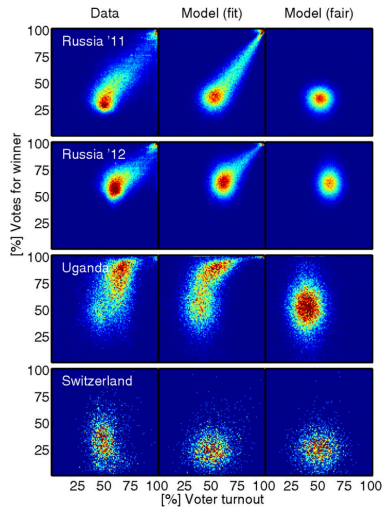
Figure 1 is reprinted examples from the referenced National Academy of Sciences paper. The actual election results in Russia, Uganda and Switzerland appear in the left column, the right column is the modeled expected appearance in a fair election with little fraud, and the middle column is the researchers’ model of the as-collected data, with any possible fraud mechanisms included.
Figure 1: NAS Paper Results (reprinted from [1])
As you can see, the election in Switzerland (assumed fair) shows a range of voter turnout, from approximately 30 – 70% across voting districts, and a similar range of votes for the winner. The Switzerland data is consistent across models, and does not show any significant irregularities.
What do the clusters mean in the Russia 2011 and 2012 elections? Of particular concern are the top right corners, showing nearly 100% turnout of voters, and nearly 100% of them voted for the winner.
Both of those events (more than 90% of registered voters turning out to vote and more than 90% of the voters voting for the winner) are statistically improbable, even for very contested elections. Election results that show a strong linear streak away from the main fingerprint lobe indicates ‘ballot stuffing,’ where ballots are added at a specific rate. Voter turnout over 100% indicates ‘extreme fraud’. [1][5]
Note that election results with ‘outliers’ – results that fall outside of expected normal voting patterns – while evidentiary indicators, are not in and of themselves definitive proof of outright fraud or malfeasance. For example, in rare but extreme cases, where the electorate is very split and the split closely follows the geographic boundaries between voting precincts, we could see multiple overlapping Gaussian lobes in the 2D image. Even in that rare case, there should not be distinct structures visible in the election fingerprint, linear streaks, overly skewed or smeared distributions, or exceedingly high turnout or vote share percentages. Additional reviews of voting patterns and election results should be conducted whenever deviations from normal patterns occur in an election.
Additionally it should be noted that “the absence of evidence is not the evidence of absence”: Election Fingerprints that look otherwise normal might still have underlying issues that are not readily apparent with this view of the data.
Results on 2024 VA March Primaries:
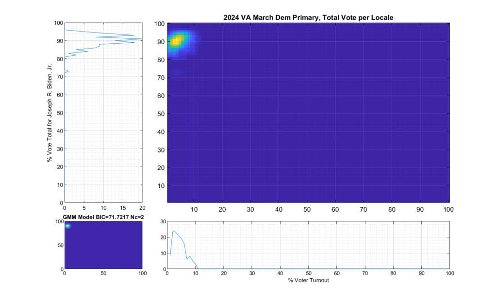
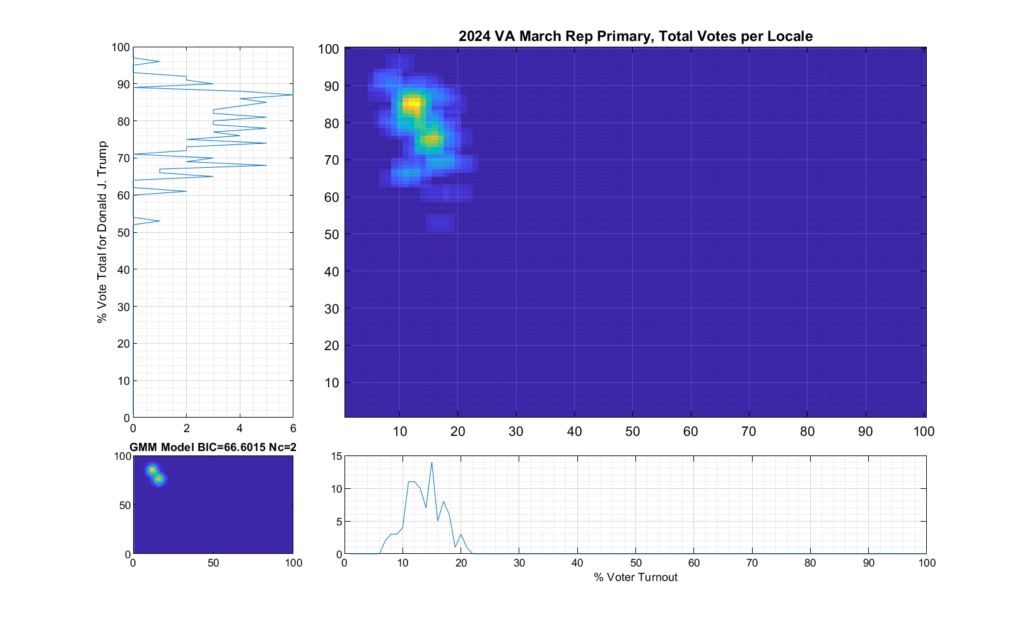
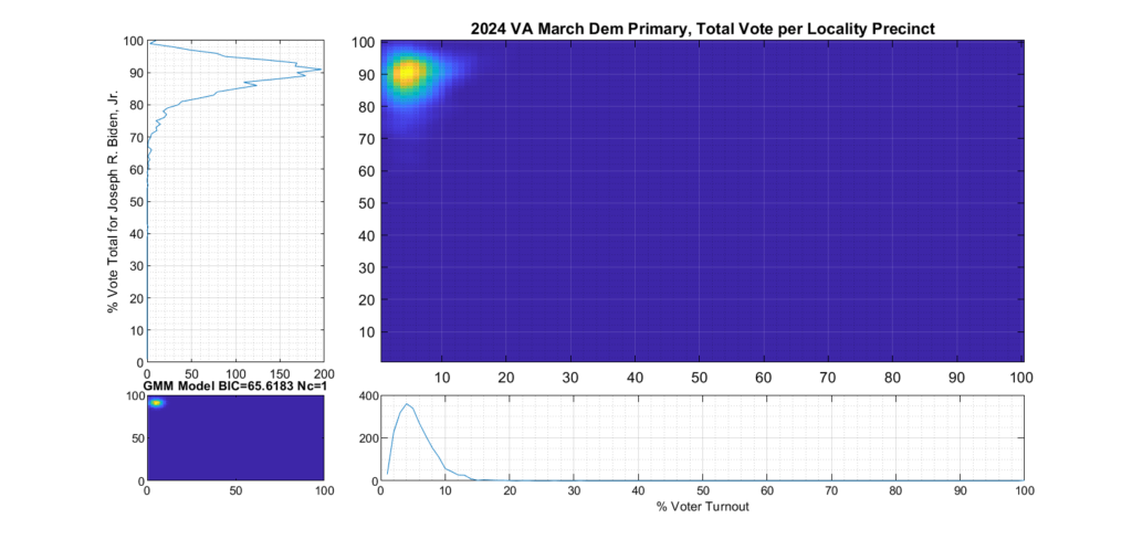
Figure 2 and Figure 3 are the computed election fingerprints for the Democratic and Republican VA 2024 March Primaries, respectively. They were computed according to the NAS paper and using official state reported voter turnout and votes for the statewide winner and reported per voting Locality with combined In-Person Early, Election Day, Absentee and Provisional votes. Figures 4 and 5 perform the same process, except each data point is generated per individual precinct in a locality. The color scale moves from precincts with low counts as deep blue, to precincts with high numbers represented as bright yellow. Note that a small blurring filter was applied to the computed image for ease of viewing small isolated Locality or Precinct results.
The upper right inset in each graphic image was computed per the NAS paper; the bottom left inset shows what an idealized model of the data could or should look like, based on the reported voter turnout and vote share for the winner. This ideal model is allowed to have up to 3 Gaussian lobes based on the peak locations and standard deviations in the reported results. The top-left and bottom-right inset plots show the sum of the rows and columns of the fingerprint image. The top-left graph corresponds to the sum of the rows in the upper right image and is the histogram of the vote share for the winner across precincts. The bottom right graph shows the sum of the columns of the upper right image, and is the histogram of the percentage turnout across voting localities.
Figure 2 Democratic primary, accumulated per Locality:
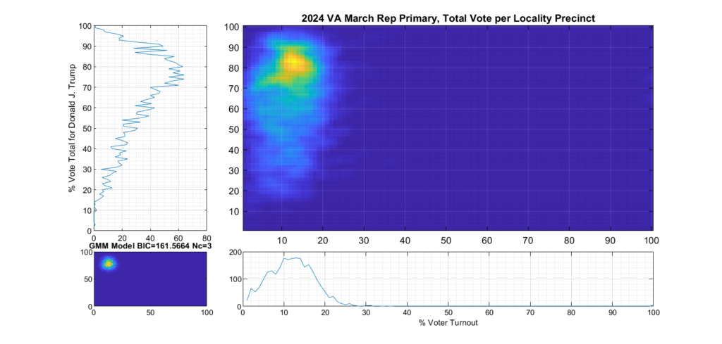
Figure 3 Republican primary, accumulated per Locality:
Figure 4 Democratic primary, accumulated per Precinct:
Figure 5 Republican primary, accumulated per Precinct:
Analysis:
As can be seen in Figure 2 and 4, the Democratic primary fingerprint looks to fall within expected normal distribution. Even though the total vote share for the winner (Biden) is up around 90%, this was not unexpected given the current set of contestants and the fact that Biden is the incumbent.
The Republican primary results, as shown in Figure 3 and 5, show significant “smearing” of the percent of total vote share for the winner. The percent of voter turnout (x-axis) does however show a near Gaussian distribution, which is what one would expect. The republican primary data does not show the linear streaking pattern that the authors in [1] correlate with extreme fraud, but significant smearing of the distribution is observed.
A consideration that might partially explain this smearing of the histogram, is that there was at least 17% of “crossover voters” who historically lean Democrat but voted in the Republican primary (see here for more information). Multiple news reports and exit polling suggest that this was due in part to loosely organized efforts by the opposing party to cast “Protest Votes” and artificially inflate the challenger (Haley) and dilute the expected (Trump) margin of victory for the winner, with no intention of supporting a Republican candidate in the General Election. (This is completely legal in VA, by the way, as VA does not require by-party voter registration.)
If we categorize each locality as being either Democratic or Republican leaning based on the average results of the last four presidential elections, and then split the computation of the per precinct results into separate parts accordingly, we can see this phenomenon much clearer.
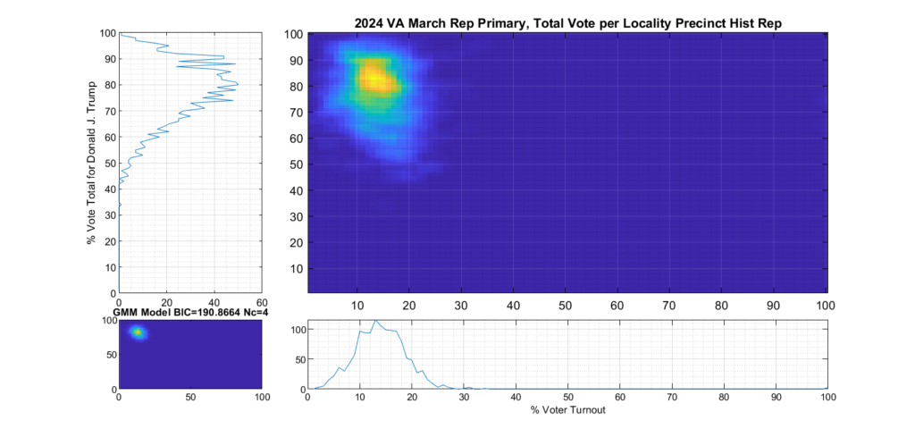
Figure 6 shows the per-precinct results for only those locality precincts that belong to historic Republican leaning localities. It depicts a much tighter distribution and has much less smearing or blurring of the distribution tails. We can see from the data that Republican base in historically Republican leaning localities seems solidly behind candidate Trump.
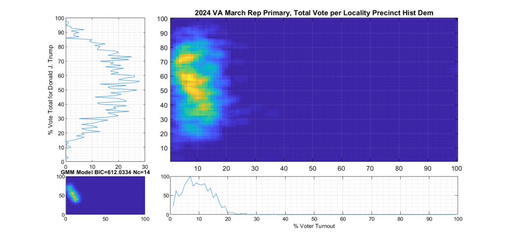
Figure 7 shows the per-precinct results for only those locality precincts that belong to historic Democratic leaning localities. It can clearly be seen by comparing the two plots that the major contributor to the spread of the total republican primary distribution is the votes from historically Democratic leaning localities.
Figure 6 Republican primary, accumulated per Precinct in Republican leaning localities:
Figure 7 Republican primary, accumulated per Precinct in Democratic leaning localities:
References:
[1] “Statistical detection of election irregularities” Peter Klimek, Yuri Yegorov, Rudolf Hanel, Stefan Thurner Proceedings of the National Academy of Sciences Oct 2012, 109 (41) 16469-16473; DOI: 10.1073/pnas.1210722109 (https://www.pnas.org/content/109/41/16469)
[5] Mebane, Walter R. and Kalinin, Kirill, Comparative Election Fraud Detection (2009). APSA 2009 Toronto Meeting Paper, Available at SSRN: https://ssrn.com/abstract=1450078
The below is based on the discussion of “Single Transferrable Vote” (“STV”) methods in [1], published in 1977. STV has more recently been called “Ranked Choice Voting” (RCV) or “Instant Runoff Voting” (IRF), among other names, by lobbying groups that are currently pushing for its incorporation into our voting systems. Irrespective of the name used, it represents a family of voting methods, with slightly different variants depending on how votes are removed and/or redistributed in each successive round of voting. [2][5]
What does STV/RCV/IRV entail, in general:
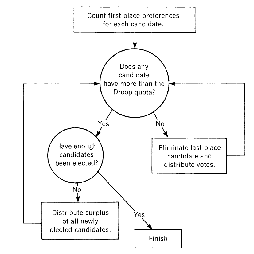
The core system is a proportional voting system, where voters are required to rank order their preferred candidate selections and all ballots are collected and centralized tabulation is performed in multiple rounds until winner(s), or candidates that have support above a specified quota (or “threshold”), are allocated.
A common definition of the quota utilized in STL/RCV/IRV systems is the “Droop quota”, and is defined as:
q = FLOOR( # of Voters / (# of Seats + 1) + 1)
In a given round the candidate with the least support is eliminated from further evaluation. Surplus votes from candidates that go over the droop threshold and votes from eliminated candidates can be distributed amongst remaining candidates for subsequent rounds. Surplus vote distribution is only applicable when multiple winners are allowed in a contest.
Vote allocation procedure for STV/RCV/IRV. Reprinted from [1].
The arguments used to support and push for RCV have not significantly changed since the time that the original paper was published, but the terms and language utilized have been modified. The authors note that much of the rationale in pushing for STV was centered around the ideas of inclusivity and making sure voters are able to cast “effective” ballots.
“Modem proponents emphasize the system’s effective representation of minorities, its sensitivity and accuracy in ‘measuring changes in popular will,’ and its tendency to encourage independent (nonparty line) voting.”
Doron, G., & Kronick, R. (1977) [1]
The same arguments have been recently repeated and pushed to legislators and the media. The name has changed from “Single Transferrable Vote” to “Ranked Choice Voting” or “Instant Runoff Voting”, but the argument remains largely the same, as can be seen by simply visiting the websites and promotional material for any of the current groups that are lobbying for RCV to be incorporated [3][4].
The issue pointed out by Doron & Kronick:
The authors in [1] note that the STV/RCV/IRV system allows for a “perversion” (their words, not mine) whereby a candidates chances to be selected as a winner can potentially be negatively impacted even when receiving increased support.
“… a function that permitted an increased vote for a candidate to cause a decline in that candidate’s rank in the social ordering-would probably strike most of us as a rather absurd, even perverse, method of arriving at a social choice. Consequently, some writers refer to this condition as the ‘Non-Perversity’ condition. All of the democratic social choice functions that have been considered in the literature were assumed to guarantee this condition, but the Single Transferrable Vote system does not.”
Doron, G., & Kronick, R. (1977) [1]
The authors present a hypothetical example to demonstrate the issue. Suppose we have 3 candidates (Candidate X, Candidate Y, Candidate Z) and two different voting groups, which we will refer to as group D and D’. Both D and D’ are fairly similar and only disagree on the relative ranking of two specific candidates.
In the tables below, recreated from [1], the only difference in the two voting group selections is that candidate X receives more support than candidate Y in group D’. However, if using the voting rules as described above candidate X wins in D, and loses in D’ even though X has increased support in D’.
# of Voters
First Choice
Second Choice
Third Choice
6
X
Y
Z
2
Y
X
Z
4
Y
Z
X
5
Z
X
Y
Voting group D selections. Reprinted from [1].
# of Voters
First Choice
Second Choice
Third Choice
6
X
Y
Z
2
X
Y
Z
4
Y
Z
X
5
Z
X
Y
Voting group D’ selections. Reprinted from [1].
There are 17 voters in each case, and only 1 seat available. Therefore, the Droop quota/threshold is 9 votes required in order to declare a winner.
In group D it is candidate Z that has the least amount of votes in the first round and is eliminated, therefore advancing 5 second-choice votes for X into the next round. Candidate X passes the threshold and wins in the second round.
In group D’, where candidate X received more support than candidate Y, it is candidate Y that has the least amount of votes in the first round and is eliminated, therefore advancing 4 second-choice votes for Z into the next round. Candidate Z then passes the threshold and wins in the second round.
Bibliography:
Doron, G., & Kronick, R. (1977). Single Transferrable Vote: An Example of a Perverse Social Choice Function. American Journal of Political Science, 21(2), 303–311. https://doi.org/10.2307/2110496
Brandt F, Conitzer V, Endriss U, Lang J, Procaccia AD, eds. Handbook of Computational Social Choice. Cambridge: Cambridge University Press; 2016. https://doi.org/10.1017/CBO9781107446984
After reading through the press release we decided to independently try to verify the claims in the release. Note that an analysis like this has been on our list of things-to-do, but there are only so many hours in the day! The fact this press release was issued gave us a well deserved prod to complete this analysis.
EPEC has purchased the entire statewide registered voter list data from the VA Department of Elections (ELECT) and has current records as of 2023-08-01. Eligible parties can purchase data from ELECT via their website here.
The necessary data from the US Census office can be downloaded here and included the estimates of the eligible voting age citizens in each county. From the documentation on the census site, the “cvap_est” field in the census data represents “The rounded estimate of the total number of United States citizens 18 years of age or older for that geographic area and group.”
It is therefore a straightforward process to accumulate the number of registrant records in each county, as well as accumulating the number of eligible voting age citizens and compute the registration percent “REG_PCT” as (# Registered / # Eligible * 100). The below table has the results of this direct computation for each county.
The results are only slightly different than the results presented by Honest Elections Project, but still show significant issues with 38 counties being over 100%.
Adjusting for population growth since 2020 census
As the census redistricting data is circa 2020, and the eligible voter data was estimated for 2021, we can attempt to account for population shifts since the 2020 census data was collected and the voter eligibility data was computed. The US Census bureau also makes available the estimates of population growth by county year-over-year since the date of the last census here, which we can use to find the recent rates of growth or decline for each county. We can then use these rates to adjust the number of eligible voter estimates to scale with the most recent rates of population change. This is admittedly an approximation and assumes a linear relationship, but it is arguably better than taking the 2020 census and 2021 eligible voter estimates and applying them directly to the latest (2023) RVL.
The REG_PCT_ADJ column in the table below represents this adjusted estimate.
Active vs inactive registrations
An additional consideration that can be made with this data, is to attempt to consider only “Active” voter registrations vs registrations with any status assigned. Note that “Inactive” voter registrations can be immediately returned to “Active” status by simply having any type of interaction with the department of elections (or through DMV, etc), and the registrant will then be allowed to vote. Because of this easy ability to change “Inactive” records to “Active”, it is most appropriate (IMO) to include them in this analysis. However, for completeness, and in order to bound the scope of the issue, the corresponding REG_PCT_ACTIVE and REG_PCT_ADJ_ACTIVE columns have also been computed which only consider “Active” voters.
Results
Even the most forgiving analysis we could compute with the official data from US Census and VA ELECT, which only considers active voters and attempts to adjust for population change since the census, still results in multiple (6) counties in VA having more than 100% registered voters than eligible voters, and many counties that had over 90%.
The most appropriate metric to consider, in my opinion, is the Adjusted and either Active or Inactive status results, as inactive status registrations can still be converted to active status and voted. There were 36 localities with over 100% in this category and 59 between 90% and 100%. There are 133 voting localities in total in VA.
The summary tabulated data and graphics for each of the methods of analyzing the data is presented below.
One thing that I have been asked about repeatedly is if there is any sort of patterns in the assignment of voter ID numbers in the VA data. Specifically, I’ve been asked repeatedly if I’ve found any similar pattern to what AuditNY has found in the NY data. It’s not something that I have looked at in depth previously due mostly to lack of time, and because VA is setup very differently than NY, so a direct comparison or attempt to replicate the AuditNY findings in VA isn’t as straightforward as one would hope.
The NY data uses a different Voter ID number for counties vs at the state level, which is the “Rosetta Stone” that was needed for the NY team to understand the algorithms that were used to assign voter ID numbers, and in turn discover some very (ahem) “interesting” patterns in the data. VA doesn’t have such a system and only uses a single voter ID number throughout the state and local jurisdictions.
Well … while my other machine is busy crunching on the string distance computations, I figured I’d take a crack at looking at the distribution of the Voter ID numbers in the VA Registered Voter List (RVL) and just see what I find.
To start with, here is a simple scatter plot of the Voter ID numbers vs the Registration date for each record in the 2023-07-01 RVL. From the zoomed out plot it is readily apparent that there must have been a change in the algorithm that was used to assign voter identification numbers sometime around 2007, which coincides nicely with the introduction of the current Virginia Election and Registration Information System (VERIS) system.
From a high level, it appears that the previous assignment algorithm broke the universe of possible ID numbers up into discrete ranges and assigned IDs within those ranges, but favoring the bottom of each range. This would be a logical explanation for the banded structure we see pre-2007. The new assignment algorithm post-2007 looks to be using a much more randomized approach. Nothing strange about that. As computing systems have gotten better and security has become more of a concern over the years there have been many systems that migrated to more randomized assignments of identification numbers.
Looking at a zoomed in block of the post-2007 “randomized” ID assignments we can see some of the normal variability that we would expect to see in the election cycles. We see that we have a high density of new assignments around November of 2016 and 2020, with a low density section of assignments correlated to the COVID-19 lockdowns. There are short periods where it looks like there were lulls in the assignment of voter ID’s, these are perhaps due to holidays or maintenance periods, or related to the legal requirements to “freeze” the voter rolls 30 days before any election (primaries, runoffs, etc). Note that VA now has same day voter registration as of the laws passed by the previous democratic super-majority that went into affect in 2022, so going forward we would likely see these “blackout periods” be significantly reduced.
We can see more clearly the banded assignment structure of the pre-2007 entries by zooming in on a smaller section of the plot, as shown below. It’s harder to make out in this banded structure, but we still see similar patterns of density changes presumably due to the natural election cycles, holidays, maintenance periods, legally required registration lockouts periods, etc. We can also see the “bucketing” of ID numbers into distinct bands, with the bias of numbers filling the lower section of each band.
All of that looks unremarkable and seems to make sense to me … however … if we zoom into the Voter ID address range of around [900,000,000 to 920,000,000] we do see something that catches my curiosity. We see the existence of the same banded structure as above between 900,000,000 and 915,000,000 AND pre-2007, but there is another band of assignments super-imposed on the entire date range of the RVL. This band does not seem to be affected by the introduction of the VERIS system (presumably), which is very interesting. There is also what looks like to be a vertical high-density band between 2007 and 2010 that extends along the entire vertical axis, but we only see it once we zoom in to the VERIS transition period.
The horizontal band that extends across all date ranges only exists in the [~915,000,000 to ~920,000,000] ID range. It trails off in density pre ~1993, but it exists throughout the full registration date range. I will note that the “Motor Voter” National Voter Registration Act (NVRA) was implemented in 1993, so perhaps these are a reserved universe block for DMV (or other externally provided) registrations? (That’s a guess, but an educated one.)
A plausible explanation I can imagine for the distinct high density band between 2007-2010 is that this might be related to how the VERIS system was implemented and brought into service, and there was some sort of update around 2010 that made correction to its internal algorithms. (But that is just a guess.) That still wouldn’t entirely explain the huge change in the density of new registrants added to the rolls.
Another, or additional, explanation might be that when VERIS came online there were a number of registrants that had their Voter ID number regenerated and/or their registration date field updated as part of the rollout of the new VERIS software. Meaning that while VERIS was coming online and handling the normal amount of new real registrations, it was also moving/updating a large number of historic registrations, which would account for the higher density as VERIS became the system of record. That seems to be a poor systems administration and design choice, in my opinion, as it makes inaccurate those moved registrant records by giving them a false registration date. However, if that was the case, and VERIS was resetting registration dates as it ingested voter records into its databases, why do we see any records with pre-2007 registration dates at all? (This is again, merely an educated guess on my part, so take with a grain of salt.)
Incorporating the identification of cloned registrations
In attempting to incorporate some of my early results on the most recent RVL data doing duplicate record identification (technically they are “cloned” records, as “duplicates” would have the same voter ID numbers. This was pointed out to me a few days ago.) on this dataset, I did a scatter plot of only those records that had an identified exact match of (FullName +DOB) to other records in the dataset, but with unique Voter ID numbers. The scatter plot of those records is shown below, and we can see that there is a distinct ~horizontal cluster of records that aligns with the 915M – 920M ID band and pre-2007. In the post-2007 block we see the cloned records do not seem to be totally randomly distributed, but have a bias towards the lower right of the graph.
Superimposing the two plots produces the following, with the red indicating the records with identified Full Name + DOB string matches.
Zooming in to take a closer look at the 915M-920M band again, gives the following:
It is curious that there seems to be an alignment of the exact Full Name + DOB matching records with the 915M-920M, pre-2007 ID band. Post-2007 the exact cloned matches have a less structured distribution throughout the data, but they do seem to cluster around the lower right.
If the cloned records were simply due to random data entry errors, etc. I would expect to see sporadic red datapoints distributed “salt-n-pepper” style throughout the entirety of the area covered by the blue data. There might be some argument to be made for there being a bias of more of the red data points to the right side of the plot, as officials have not yet had time to “catch” or “clean-up” erroneous entries, but there is little reason to have linear features, or to have a bias for lower ID numbers in the vertical axis.
I am continuing to investigate this data, but as of right now all I can tell you is that … yes, there does seem to be interesting patterns in the way Voter IDs are assigned in VA, especially with records that have already been found and flagged to be problematic (clones).