Per request by a reviewer of my most recent election irregularities report in VA (here), here’s a little more technical detail as to how the “ideal” model is computed in accordance with the original 2012 National Academy of Sciences paper that I based this work off of.
The generalized summary in my report for VA reads as follows:
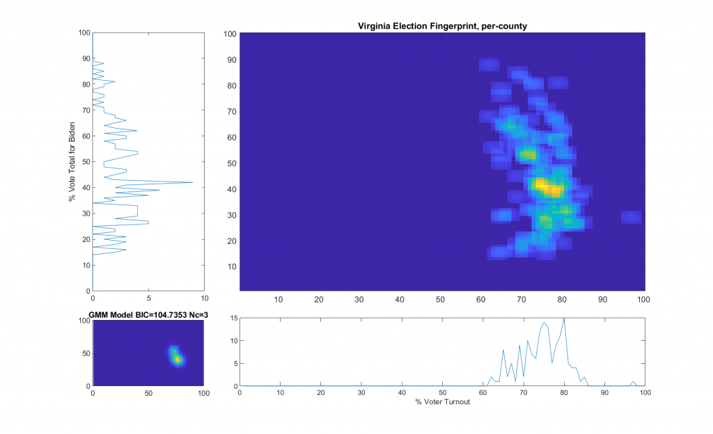
“The upper right image was computed per the NAS paper; the bottom left image shows what an idealized model of the data could or should look like, based on the reported voter turnout and vote share for the winner. This ideal model is allowed to have up to 3 Gaussian lobes based on the peak locations and standard deviations in the reported Virginia results.”
While that description is absolutely accurate, it glosses over some of the implementation as I didn’t want the reader to go all glassy-eyed on me! A more explicit technical definition is as follows: All of the localized maximal peaks in the 2D histogram that are above pThresh (~= 0.7) x the value of the global maximum peak are used as the centroids of a Gaussian Mixture model, with shared covariance matrix equal to 1.5 x sqrt of the covariance matrix of all of the data points. (Thats a lot of mathematics packed into one sentence, but its accurate!) In the case of the VA per county per cong district data this give us either 2 or 3 peaks dependent on the value that is used for the pThresh threshold. The value of 0.7 was chosen after observing results from multiple states data that I have been doing fingerprint analysis on. The MATLAB imregionalmax(…) function from the Image Processing Toolbox is used to find the candidate localized peaks, and the gmdistribution(…) function from the Statistics toolbox generated the final idealized model.
% HBf is the 2D Histogram image
BW = imregionalmax(HBf);
v = HBf(BW);
[r,c] = find(BW.*HBf >=  max(v(:))*pThresh);
mu = [r,c];
s = 1.5;

cv = diag(diag(s*sqrt(cov(rawData))));
GMModel = gmdistribution(mu,cv);
The end result of this is shown below (bottom left) with the Bayesian Information Criterion (BIC) and number of Gaussian components listed in the title of the bottom left “ideal” plot.