Note: For background information, please see my introduction to Cast Vote Records processing and theory here: Statistical Detection of Irregularities via Cast Vote Records.
Since I posted my initial analysis of the Henrico CVR data, one comment was made to me by a member of the Texas election integrity group I have been working with: We have been assuming, based on vendor documentation and the laws and requirements in various states, that when a cast vote record is produced by vendor software the results are sorted by the time the ballot was recorded onto a scanner. However, when looking at the results that we’ve been getting so far and trying to figure out plausible explanations for what we were seeing, he realized it might be the case that the ordering of the CVR entries are being done by both time AND USB stick grouping (which is usually associated with a specific scanner or precinct) but then simply concatenating all of those results together.
While there isn’t enough information in the Henrico CVR files to breakout the entries by USB/Scanner, and the Henrico data has record ID numbers instead of actual timestamps, there is enough information to break out them by Precinct, District and Race, with the exception of the Central Absentee Precincts (CAP) entries where we can only break them out by district given the metadata alone. However, with some careful MATLAB magic I was able to cluster the results marked as just “CAP” into at least 5 different sub-groupings that are statistically distinct. (I used an exponential moving average to discover the boundaries between groupings, and looking at the crossover points in vote share.) I then relabeled the entries with the corresponding “CAP 1”, “CAP 2”, … , “CAP 5” labels as appropriate. My previous analysis was only broken out by Race ID and CAP/Non-CAP/Provisional category.
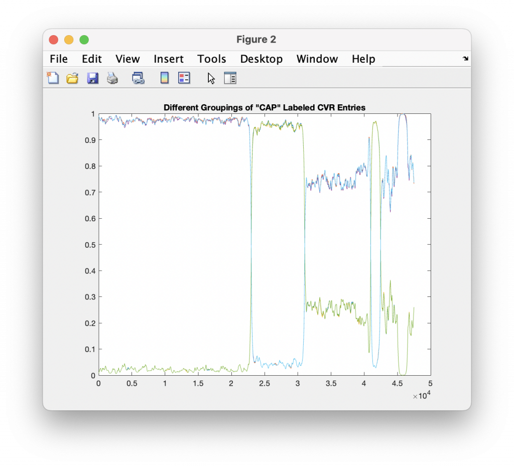
Processing in this manner makes the individual distributions look much cleaner, so I think this does confirm that there is not a true sequential ordering in the CVR files coming out of the vendor software packages. (If they would just give us the dang timestamps … this would be a lot easier!)
I have also added a bit more rigor to the statistics outlier detection by adding plots of the length of observed runs (e.g. how many “heads” did we get in a row?) as we move through the entries, as well as the plot of the probability of this number of consecutive tosses occurring. We compute this probability for K consecutive draws using the rules of statistical independence, which is P([a,a,a,a]) = P(a) x P(a) x P(a) x P(a) = P(a)^4. Therefore the probability of getting 4 “heads” in a row with a hypothetical 53/47 weighted coin would be .53^4 = 0.0789. There are also plotted lines for a probability 1/#Ballots for reference.
Results
The good news is that this method of slicing the data and assuming that the Vendor is simply concatenating USB drives seems to produce much tighter results that look to obey the expected IID distributions. Breaking up the data this way resulted in no plot breaking the +/- 3/sqrt(N-1) boundaries, but there still are a few interesting datapoints that we can observe.
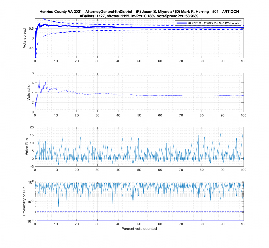
In the plot below we have the Attorney Generals race in the 4th district from precinct 501 – Antioch. This is a district that Miyares won handily 77%/23%. We see that the top plot of the cumulative spread is nicely bounded by the +/- 3/sqrt(N-1) lines. The second plot from the top gives the vote ratio in order to compare with the work that Draza Smith, Jeff O’Donnell and others are doing with CVR’s over at Ordros.com. The second from bottom plot gives the number k of consecutive ballots (in either candidates favor) that have been seen at each moment in the counting process. And the bottom plot raises either the 77% or 23% overall probability to the k-th power to determine the probability associated with pulling that many consecutive Miyares or Herring ballots from an IID distribution. The most consecutive ballots Miyares received in a row was just over 15, which had a .77^15 = 0.0198 or 1.98% chance of occurring. The most consecutive ballots Herring received was about 4, which equates to a probability of occurrence of .23^4 = 0.0028 or 0.28% chance. The dotted line on the bottom plot is referenced at 1/N, and the solid line is referenced at 0.01%.
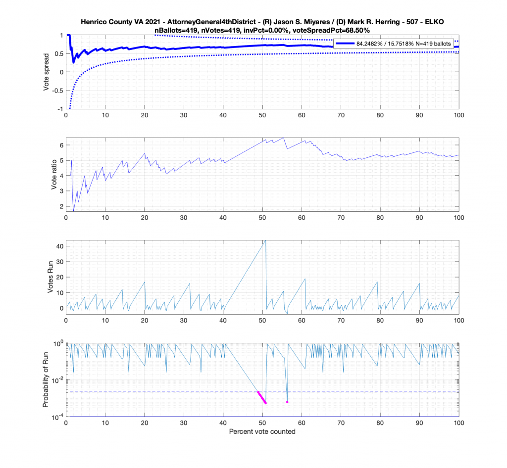
But let’s now take a look at another plot for the Miyares contest in another blowout locality with 84% / 16% for Miyares. The +/- 3/sqrt(N-1) limit nicely bounds our ballot distribution again. There is, however, an interesting block of 44 consecutive ballots for Miyares about halfway through the processing of ballots. This equates to .84^44 = 0.0004659 or a 0.04659% chance of occurrence from an IID distribution. Close to this peak is a run of 4 ballots for Herring which doesn’t sound like much, but given the 84% / 16% split, the probability of occurrence for that small run is .16^4 = 0.0006554 or 0.06554%!
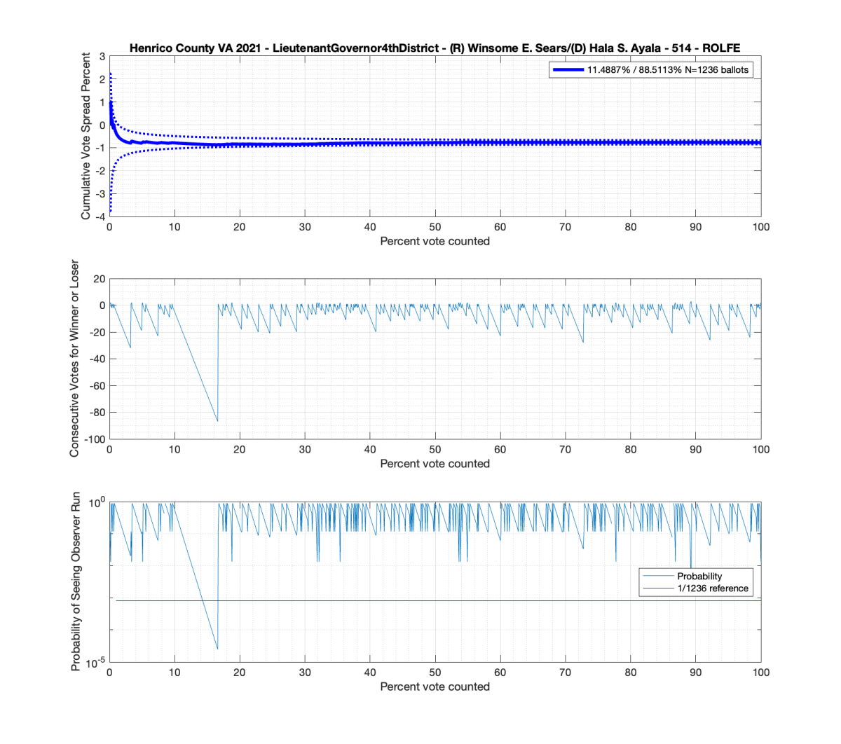
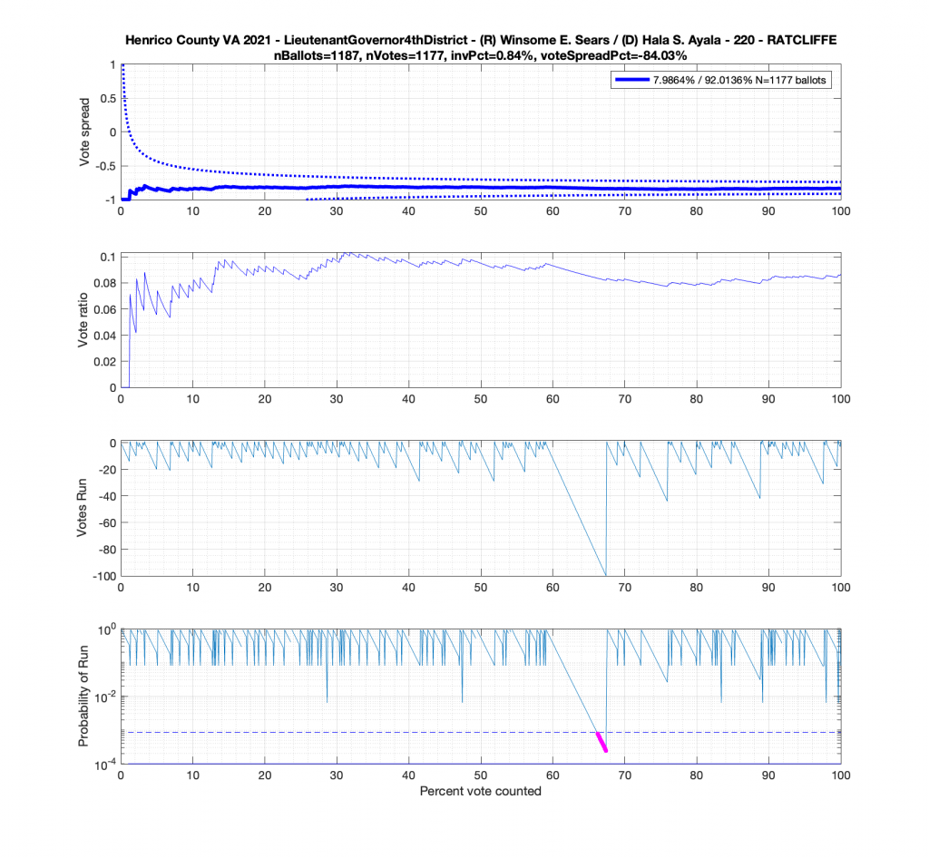
Moving to the Lt. Governors race we see an interesting phenomenon where where Ayala received a sudden 100 consecutive votes a little over midway through the counting process. Now granted, this was a landslide district for Ayala, but this still equates to a .92^100 = 0.000239 or 0.0239% chance of occurrence.
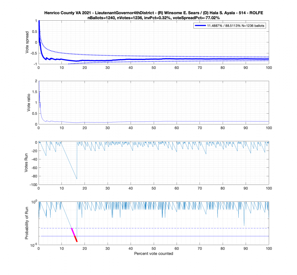
And here’s another large block of contiguous Ayala ballots equating to about .89^84 = 0.00005607 or 0.0056% chance of occurrence.
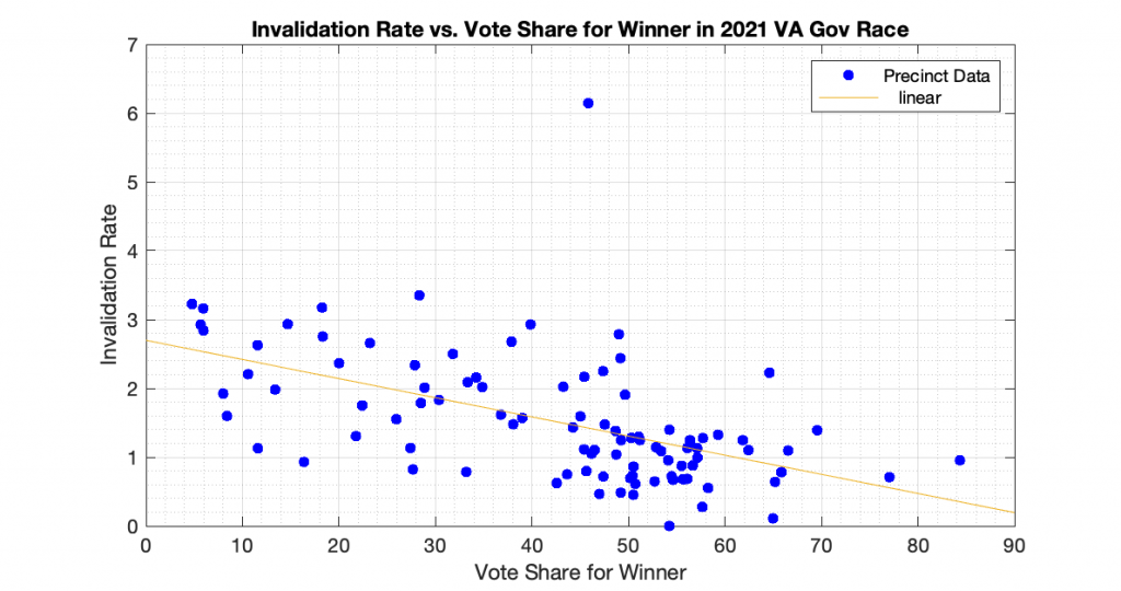
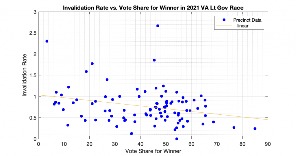
Tests for Differential Invalidation (added 2022-09-19):
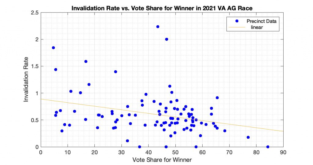
“Differential invalidation” takes place when the ballots of one candidate or position are invalidated at a higher rate than for other candidates or positions. With this dataset we know how many ballots were cast, and how many ballots had incomplete or invalid results (no recorded vote in the cvr, but the ballot record exists) for the 3 statewide races. In accordance with the techniques presented in [1] and [2], I computed the plots of the Invalidation Rate vs the Percent Vote Share for the Winner in an attempt to observe if there looks to be any evidence of Differential Invalidation ([1], ch 6). This is similar to the techniques presented in [2], which I used previously to produce my election fingerprint plots and analysis that plotted the 2D histograms of the vote share for the winner vs the turnout percentage.
The generated the invalidation rate plots for the Gov, Lt Gov and AG races statewide in VA 2021 are below. Each plot below is representing one of the statewide races, and each dot is representing the ballots from a specific precinct. The x axis is the percent vote share for the winner, and the y axis is computed as 100 – 100 * Nvotes / Nballots. All three show a small but statistically significant linear trend and evidence of differential invalidation. The linear regression trendlines have been computed and superimposed on the data points in each graph.
To echo the warning from [1]: a differential invalidation rate does not directly indicate any sort of fraud. It indicates an unfairness or inequality in the rate of incomplete or invalid ballots conditioned on candidate choice. While it could be caused by fraud, it could also be caused by confusing ballot layout, or socio-economic issues, etc.
Full Results Download
References
- [1] Forsberg, O.J. (2020). Understanding Elections through Statistics: Polling, Prediction, and Testing (1st ed.). Chapman and Hall/CRC. https://doi.org/10.1201/9781003019695
- [2] Klimek, Peter & Yegorov, Yuri & Hanel, Rudolf & Thurner, Stefan. (2012). Statistical Detection of Systematic Election Irregularities. Proceedings of the National Academy of Sciences of the United States of America. 109. 16469-73. https://doi.org/10.1073/pnas.1210722109.